---
title: "Extravascular (Oral/SC) Examples"
---
```{r setup, include=FALSE}
library(PKNCA)
library(dplyr)
library(ggplot2)
conflicted::conflicts_prefer(dplyr::filter, dplyr::select, .quiet = TRUE)
```
## The EV dataset: Theophylline
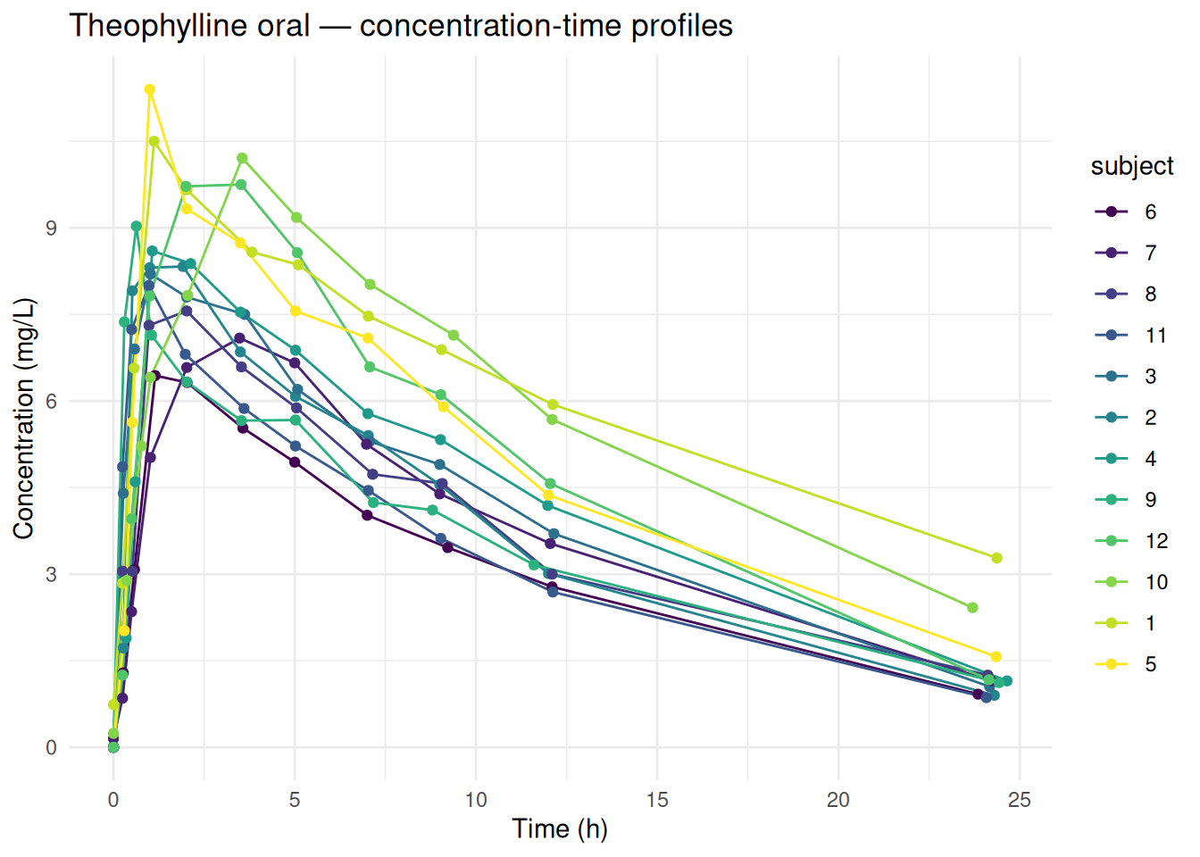
We use `datasets::Theoph` — oral theophylline (bronchodilator) in 12 subjects, sampled over 25 hours after a single oral dose.
```{r}
head(Theoph)
str(Theoph)
```
Columns: `Subject`, `Wt` (body weight, kg), `Dose` (mg/kg), `Time` (h), `conc` (mg/L).
```{r}
# Prepare concentration data
d_conc <- as.data.frame(Theoph) |>
  rename(time = Time, subject = Subject, conc = conc)

# Prepare dose data: convert mg/kg to mg per subject
d_dose <- Theoph |>
  as.data.frame() |>
  group_by(Subject) |>
  summarise(dose = Dose[1] * Wt[1], .groups = "drop") |>
  rename(subject = Subject) |>
  mutate(time = 0)

# Visualize concentration profiles
ggplot(d_conc, aes(x = time, y = conc, group = subject, colour = subject)) +
  geom_line() + geom_point() +
  labs(title = "Theophylline oral — concentration-time profiles",
       x = "Time (h)", y = "Concentration (mg/L)") +
  theme_minimal()
```
The typical absorption-distribution-elimination shape is visible: concentrations rise to a peak (Tmax/Cmax) then decline.
---
## Basic extravascular analysis
```{r}
o_conc <- PKNCAconc(d_conc, conc ~ time | subject)

o_dose <- PKNCAdose(d_dose, dose ~ time | subject, route = "extravascular")

# Core EV parameters
ev_intervals <- data.frame(
  start       = 0,
  end         = Inf,
  cmax        = TRUE,
  tmax        = TRUE,
  auclast     = TRUE,
  aucinf.obs  = TRUE,
  half.life   = TRUE,
  lambda.z    = TRUE,
  cl.obs      = TRUE,   # apparent CL (= CL/F for EV)
  vz.obs      = TRUE    # apparent Vz (= Vz/F for EV)
)

o_data <- PKNCAdata(o_conc, o_dose, intervals = ev_intervals)
o_nca  <- pk.nca(o_data)

as.data.frame(o_nca) |>
  select(subject, PPTESTCD, PPORRES) |>
  arrange(subject, PPTESTCD)
```
---
## Parameter reference
### Concentration and time landmarks
| Parameter | Meaning |
|---|---|
| `cmax` | Maximum observed concentration |
| `tmax` | Time of Cmax |
| `cmin` | Minimum observed concentration in the interval |
| `tmin` | Time of the minimum observed concentration (≥ 0.12.2) |
| `tfirst` | First time with a non-zero (non-BLQ) concentration |
| `tlast` | Last time with a measurable concentration |
| `clast.obs` | Observed concentration at `tlast` |
| `clast.pred` | Predicted concentration at `tlast` (from λz fit) |
| `count_conc` | Total observations (including BLQ) |
| `count_conc_measured` | Observations above the LLOQ |
| `lambda.z.time.last` | Last timepoint used in the λz regression |
```{r}
lm_interval <- data.frame(
  start               = 0,
  end                 = Inf,
  cmax                = TRUE,
  tmax                = TRUE,
  cmin                = TRUE,
  tmin                = TRUE,
  tfirst              = TRUE,
  tlast               = TRUE,
  clast.obs           = TRUE,
  clast.pred          = TRUE,
  count_conc          = TRUE,
  count_conc_measured = TRUE
)

o_nca_lm <- pk.nca(PKNCAdata(o_conc, o_dose, intervals = lm_interval))

as.data.frame(o_nca_lm) |>
  filter(PPTESTCD %in% c("cmax","tmax","cmin","tmin","tfirst","tlast",
                          "clast.obs","clast.pred","count_conc","count_conc_measured")) |>
  select(subject, PPTESTCD, PPORRES) |>
  arrange(subject, PPTESTCD)
```
**When there are multiple peaks** (fed state, enterohepatic recirculation), the default is to return the first Tmax. Control this with `first.tmax`:
Tie-breaking for Tmin is controlled by the `first.tmin` option (PKNCA ≥ 0.12.2, default `TRUE` = return first occurrence):
```{r}
# Use the last Tmax when there are ties
o_data_lasttmax <- PKNCAdata(
  o_conc, o_dose,
  intervals = ev_intervals,
  options = list(first.tmax = FALSE)
)
```
### AUC variants
Same variants as IV, but note that for EV routes **CL and Vz are apparent** (divided by F, the bioavailability fraction):
| Parameter | Meaning |
|---|---|
| `auclast` | AUC from 0 to last measurable concentration |
| `aucinf.obs` | AUC extrapolated to ∞ (using observed Clast) |
| `aucinf.pred` | AUC extrapolated to ∞ (using predicted Clast) |
| `aucpext.obs` | % of AUCinf that is extrapolated |
| `cl.obs` | Apparent clearance = Dose / AUCinf.obs (this is CL/F) |
| `vz.obs` | Apparent volume = CL.obs / λz (this is Vz/F) |
```{r}
auc_params <- data.frame(
  start        = 0,
  end          = Inf,
  auclast      = TRUE,
  aucinf.obs   = TRUE,
  aucinf.pred  = TRUE,
  aucpext.obs  = TRUE,
  cl.obs       = TRUE
)

o_data_auc <- PKNCAdata(o_conc, o_dose, intervals = auc_params)
o_nca_auc  <- pk.nca(o_data_auc)

as.data.frame(o_nca_auc) |>
  filter(PPTESTCD %in% c("auclast", "aucinf.obs", "aucpext.obs", "cl.obs")) |>
  select(subject, PPTESTCD, PPORRES) |>
  tidyr::pivot_wider(names_from = PPTESTCD, values_from = PPORRES) |>
  arrange(subject)
```
### Half-life and λz
For EV, the terminal phase reflects elimination (not absorption) once absorption is complete. The same quality controls apply as for IV.
```{r}
hl_params <- data.frame(
  start             = 0,
  end               = Inf,
  lambda.z          = TRUE,
  half.life         = TRUE,
  lambda.z.n.points = TRUE,
  r.squared         = TRUE,
  adj.r.squared     = TRUE
)

o_data_hl <- PKNCAdata(o_conc, o_dose, intervals = hl_params)
o_nca_hl  <- pk.nca(o_data_hl)

as.data.frame(o_nca_hl) |>
  filter(PPTESTCD %in% c("half.life", "lambda.z.n.points", "adj.r.squared")) |>
  select(subject, PPTESTCD, PPORRES) |>
  arrange(subject, PPTESTCD)
```
**Allow or exclude Tmax from the terminal regression:**
By default, the Tmax point is excluded from the λz regression (absorption may still be ongoing). You can override this:
```{r}
o_data_allow_tmax <- PKNCAdata(
  o_conc, o_dose,
  intervals = hl_params,
  options = list(allow.tmax.in.half.life = TRUE)
)
```
### Lag time (tlag)
`tlag` is the time before absorption begins — the delay between dosing and the first measurable rise in concentration. Common for enteric-coated formulations or SC injections with a diffusion delay.
```{r}
o_nca_tlag <- pk.nca(PKNCAdata(o_conc, o_dose,
  intervals = data.frame(start = 0, end = Inf, tlag = TRUE, tmax = TRUE, cmax = TRUE)))

as.data.frame(o_nca_tlag) |>
  filter(PPTESTCD %in% c("tlag", "tmax", "cmax")) |>
  select(subject, PPTESTCD, PPORRES) |>
  tidyr::pivot_wider(names_from = PPTESTCD, values_from = PPORRES) |>
  arrange(subject)
```
> For the Theoph dataset tlag is 0 for all subjects (no lag). It becomes non-zero when the concentration-time profile shows a flat period after dosing before rising.
### Bioavailability (f)
`f` computes the ratio of AUC between two routes or treatments within the same subject. It requires a **reference** AUC in the grouping structure (typically set up with a treatment or period column).
```{r}
# Syntax: request f = TRUE; PKNCA computes AUC_test / AUC_reference
# Requires a grouping column that identifies test vs. reference
# Example structure (illustrative — Theoph is single-arm):
data.frame(start = 0, end = Inf, aucinf.obs = TRUE, f = FALSE)
# f = TRUE only makes sense when the data has paired test/reference periods
```
> See `?pk.calc.f` for the full setup. `f` is typically used in crossover bioequivalence studies.
### Volume at steady state (Vss)
Vss is computed from CL and MRT. For EV routes these are apparent values (divided by F).
```{r}
vss_params <- data.frame(
  start    = 0,
  end      = Inf,
  vss.obs  = TRUE,   # apparent Vss = CL.obs × MRT.obs
  vss.pred = TRUE
)

o_nca_vss <- pk.nca(PKNCAdata(o_conc, o_dose, intervals = vss_params))
as.data.frame(o_nca_vss) |>
  filter(PPTESTCD %in% c("vss.obs", "vss.pred")) |>
  select(subject, PPTESTCD, PPORRES) |>
  arrange(subject, PPTESTCD)
```
### Vss variants
For extravascular dosing, `vss.obs` and `vss.pred` are the apparent Vss (i.e., Vss/F). `vss.last` uses MRTlast instead of the extrapolated MRT.
```{r}
vss_all_params <- data.frame(
  start    = 0, end = Inf,
  vss.obs  = TRUE,
  vss.pred = TRUE,
  vss.last = TRUE
)
o_nca_vss_all <- pk.nca(PKNCAdata(o_conc, o_dose, intervals = vss_all_params))
as.data.frame(o_nca_vss_all) |>
  filter(grepl("^vss", PPTESTCD)) |>
  select(subject, PPTESTCD, PPORRES) |>
  arrange(subject, PPTESTCD)
```
### MRT variants
| Parameter | Meaning |
|---|---|
| `mrt.last` | AUMC(0–last) / AUC(0–last) |
| `mrt.obs` | AUMC(0–∞) / AUC(0–∞), observed Clast |
| `mrt.pred` | AUMC(0–∞) / AUC(0–∞), predicted Clast |
```{r}
mrt_ev_params <- data.frame(
  start    = 0, end = Inf,
  mrt.last = TRUE,
  mrt.obs  = TRUE,
  mrt.pred = TRUE
)
o_nca_mrt_ev <- pk.nca(PKNCAdata(o_conc, o_dose, intervals = mrt_ev_params))
as.data.frame(o_nca_mrt_ev) |>
  filter(grepl("^mrt", PPTESTCD)) |>
  select(subject, PPTESTCD, PPORRES) |>
  arrange(subject, PPTESTCD)
```
### Effective half-life and kel
All extravascular effective half-life and elimination rate constant variants:
| Parameter | Based on |
|---|---|
| `thalf.eff.last` | `mrt.last` |
| `thalf.eff.obs` | `mrt.obs` |
| `thalf.eff.pred` | `mrt.pred` |
| `kel.obs` | 1 / `mrt.obs` |
| `kel.pred` | 1 / `mrt.pred` |
| `kel.last` | 1 / `mrt.last` |
```{r}
eff_params <- data.frame(
  start           = 0, end = Inf,
  thalf.eff.last  = TRUE,
  thalf.eff.obs   = TRUE,
  thalf.eff.pred  = TRUE,
  kel.obs         = TRUE,
  kel.pred        = TRUE,
  kel.last        = TRUE
)

o_nca_eff <- pk.nca(PKNCAdata(o_conc, o_dose, intervals = eff_params))
as.data.frame(o_nca_eff) |>
  filter(grepl("^(thalf|kel)", PPTESTCD)) |>
  select(subject, PPTESTCD, PPORRES) |>
  arrange(subject, PPTESTCD)
```
### AUC for a specific tau (dosing interval)
For multiple-dose studies, request AUC over the dosing interval (tau):
```{r}
# Single dose, but demonstrating syntax for AUC(0-tau)
tau_interval <- data.frame(
  start      = 0,
  end        = 24,      # tau = 24 h
  auclast    = TRUE,
  cmax       = TRUE,
  tmax       = TRUE
)

o_data_tau <- PKNCAdata(o_conc, o_dose, intervals = tau_interval)
o_nca_tau  <- pk.nca(o_data_tau)
as.data.frame(o_nca_tau) |> select(subject, PPTESTCD, PPORRES)
```
---
## Imputation of missing predose concentrations
In some studies, the predose sample is missing or was not collected. PKNCA can impute a time-0 concentration before calculations.
Available built-in methods (comma-separate to chain them):
| Method | What it does |
|---|---|
| `start_predose` | Uses the last pre-interval concentration at the interval start (no sample is added if no pre-interval observation exists) |
| `start_conc0` | Sets the predose concentration to 0 unconditionally |
| `start_cmin` | Uses the minimum observed concentration as predose value |
```{r}
# Remove the time=0 observation from subject 1 to simulate missing predose
d_conc_missing <- d_conc |>
  filter(!(subject == "1" & time == 0))

o_conc_miss <- PKNCAconc(d_conc_missing, conc ~ time | subject)

# With imputation: add back a 0 at time 0
o_data_imputed <- PKNCAdata(
  o_conc_miss, o_dose,
  intervals = ev_intervals,
  impute = "start_predose"
)

o_nca_imputed <- pk.nca(o_data_imputed)
# Compare subject 1 AUC with and without imputation
bind_rows(
  as.data.frame(o_nca) |> filter(subject == "1", PPTESTCD == "auclast") |> mutate(version = "original"),
  as.data.frame(o_nca_imputed) |> filter(subject == "1", PPTESTCD == "auclast") |> mutate(version = "imputed")
) |>
  select(version, PPTESTCD, PPORRES)
```
**Per-interval imputation** — apply different methods to different calculation windows:
```{r}
# Intervals with an "impute" column specifying method per row
d_intervals_impute <- data.frame(
  start   = 0,
  end     = Inf,
  auclast = TRUE,
  impute  = "start_predose"
)

o_data_per_interval <- PKNCAdata(
  o_conc_miss, o_dose,
  intervals = d_intervals_impute,
  impute = "impute"   # tells PKNCA to look in the intervals column named "impute"
)
```
---
## Bioavailability
Bioavailability (F) compares AUC from the EV route to AUC from an IV reference.
PKNCA calculates this if you supply both an IV and an EV `PKNCAresults` object.
```{r}
# IV reference (using Indometh as stand-in — illustrative syntax only)
d_iv_conc <- as.data.frame(Indometh)
d_iv_dose <- data.frame(Subject = unique(d_iv_conc$Subject), dose = 25, time = 0)

o_iv_conc <- PKNCAconc(d_iv_conc, conc ~ time | Subject)
o_iv_dose <- PKNCAdose(d_iv_dose, dose ~ time | Subject, route = "intravascular")
o_iv_data <- PKNCAdata(o_iv_conc, o_iv_dose, intervals = data.frame(
  start = 0, end = Inf, aucinf.obs = TRUE
))
o_iv_nca <- pk.nca(o_iv_data)
# pk.business.rule: bioavailability is computed via pk.calc.f()
# Use pk.calc.f() directly when you have matched IV and EV AUCs
iv_aucinf <- as.data.frame(o_iv_nca) |>
  filter(PPTESTCD == "aucinf.obs") |>
  summarise(mean_aucinf = mean(PPORRES)) |>
  pull(mean_aucinf)

ev_aucinf <- as.data.frame(o_nca_auc) |>
  filter(PPTESTCD == "aucinf.obs") |>
  summarise(mean_aucinf = mean(PPORRES)) |>
  pull(mean_aucinf)

# F (%) = (AUC_ev / Dose_ev) / (AUC_iv / Dose_iv) * 100
# These datasets use different drugs, so this is illustrative only:
cat("Illustrative F calculation:\n")
cat(sprintf(" IV AUCinf (mean): %.2f\n", iv_aucinf))
cat(sprintf(" EV AUCinf (mean): %.2f\n", ev_aucinf))
```
> For a real bioavailability study, subjects would receive both IV and EV treatments, and `pk.calc.f()` handles the ratio calculation accounting for dose scaling.
---
## Multiple-dose / steady-state
For multiple-dose studies, specify the dosing interval in your intervals data frame. PKNCA will compute accumulation-relevant parameters:
```{r}
# Steady-state interval parameters
ss_params <- c("cmax", "cmin", "tmax", "auclast", "half.life", "lambda.z")

ss_intervals <- data.frame(
  start  = 0,
  end    = 24,
  cmax   = TRUE,
  cmin   = TRUE,
  tmax   = TRUE,
  auclast = TRUE
)

o_data_ss <- PKNCAdata(o_conc, o_dose, intervals = ss_intervals)
o_nca_ss  <- pk.nca(o_data_ss)

as.data.frame(o_nca_ss) |>
  select(subject, PPTESTCD, PPORRES) |>
  arrange(subject, PPTESTCD)
```
---
## Excluding observations
Mark individual time points to exclude (e.g., emesis within 2× Tmax, suspected contamination):
```{r}
d_conc_excl <- d_conc |>
  mutate(
    exclude_reason = ifelse(subject == "5" & time == 7.02,
                            "vomiting within 2h of Tmax", NA_character_)
  )

o_conc_excl <- PKNCAconc(d_conc_excl, conc ~ time | subject, exclude = "exclude_reason")

o_data_excl <- PKNCAdata(o_conc_excl, o_dose, intervals = ev_intervals)
o_nca_excl  <- pk.nca(o_data_excl)
```
Excluded points appear flagged in `as.data.frame()` output, preserving audit trail.
---
## BLQ (below limit of quantification) handling
PKNCA's `conc.blq` option controls how BLQ values (typically entered as 0) are treated:
The default is `list(first = "keep", middle = "drop", last = "keep")`:
- `first` — BLQs before the first non-BLQ concentration (keep, often a pre-dose zero)
- `middle` — BLQs sandwiched between non-BLQ values (dropped by default)
- `last` — BLQs after the last non-BLQ concentration (keep by default)
You can override globally or with positional keys:
```{r}
# Global: treat all BLQ as 0
o_data_blq_keep <- PKNCAdata(
  o_conc, o_dose,
  intervals = ev_intervals,
  options = list(conc.blq = "keep")
)

# Global: remove all BLQ values
o_data_blq_drop <- PKNCAdata(
  o_conc, o_dose,
  intervals = ev_intervals,
  options = list(conc.blq = "drop")
)

# Per-phase (before/after Tmax):
o_data_blq <- PKNCAdata(
  o_conc, o_dose,
  intervals = ev_intervals,
  options = list(
    conc.blq = list(
      before.tmax = "keep",   # keep 0s before Tmax (ascending phase)
      after.tmax  = "drop"    # drop BLQs after Tmax
    )
  )
)
```
---
## AUC integration methods
The default integration method is **lin up / log down** (linear interpolation on the ascending phase, log-linear on the descending phase). Three methods are available:
```{r}
# Method 1: linear trapezoidal (simplest)
o_data_lin <- PKNCAdata(o_conc, o_dose, intervals = ev_intervals,
                         options = list(auc.method = "linear"))

# Method 2: lin-log (log trapezoidal throughout — not recommended)
o_data_linlog <- PKNCAdata(o_conc, o_dose, intervals = ev_intervals,
                            options = list(auc.method = "lin-log"))

# Method 3: lin up/log down (default, recommended)
o_data_liuplogdown <- PKNCAdata(o_conc, o_dose, intervals = ev_intervals,
                                 options = list(auc.method = "lin up/log down"))

# Compare AUClast across methods
compare_methods <- function(label, data_obj) {
  nca <- pk.nca(data_obj)
  as.data.frame(nca) |>
    filter(PPTESTCD == "auclast") |>
    mutate(method = label) |>
    select(method, subject, PPORRES)
}

bind_rows(
  compare_methods("linear",           o_data_lin),
  compare_methods("lin up/log down",  o_data_liuplogdown)
) |>
  tidyr::pivot_wider(names_from = method, values_from = PPORRES) |>
  arrange(subject)
```
---
## Units
```{r}
units_table <- pknca_units_table(
  concu   = "mg/L",
  timeu   = "h",
  doseu   = "mg",
  amountu = "mg"
)

o_conc_u <- PKNCAconc(d_conc, conc ~ time | subject, concu = "mg/L", timeu = "h")
o_dose_u <- PKNCAdose(d_dose, dose ~ time | subject, route = "extravascular",
                      doseu = "mg", timeu = "h")
o_data_u <- PKNCAdata(o_conc_u, o_dose_u, intervals = ev_intervals, units = units_table)
o_nca_u  <- pk.nca(o_data_u)

as.data.frame(o_nca_u) |>
  filter(PPTESTCD %in% c("auclast", "aucinf.obs", "cl.obs", "half.life")) |>
  select(subject, PPTESTCD, PPORRES) |>
  arrange(subject, PPTESTCD)
```
---
## Summary
```{r}
summary(o_nca)
```
Customize for specific parameters:
```{r}
PKNCA.set.summary(
  "tmax",
  description = "median [min, max]",
  point  = median,
  spread = function(x) c(min(x), max(x))  # must return numeric; PKNCA formats the string
)

summary(o_nca)
```
---
## Full parameter list for extravascular
All extravascular-relevant parameters you can request in an interval:
```{r}
interval_cols <- get.interval.cols()
ev_relevant <- c(
  # Concentration / time landmarks
  "cmax", "tmax", "cmin", "tfirst", "tlast", "tlag",
  "clast.obs", "clast.pred", "count_conc", "count_conc_measured",
  # AUC family
  "auclast", "aucall", "aucinf.obs", "aucinf.pred",
  "aucpext.obs", "aucpext.pred",
  "aucint.last", "aucint.last.dose", "aucint.all", "aucint.all.dose",
  "aucint.inf.obs", "aucint.inf.obs.dose",
  # AUMC
  "aumclast", "aumcall", "aumcinf.obs", "aumcinf.pred",
  # Half-life / λz
  "half.life", "lambda.z", "lambda.z.n.points", "lambda.z.time.first", "lambda.z.time.last",
  "r.squared", "adj.r.squared", "span.ratio",
  # Clearance (apparent)
  "cl.obs", "cl.pred", "cl.last", "cl.all",
  # Volume (apparent)
  "vz.obs", "vz.pred", "vss.obs", "vss.pred", "vss.last",
  # MRT
  "mrt.last", "mrt.obs", "mrt.pred",
  # Effective half-life / kel
  "thalf.eff.last", "thalf.eff.obs", "thalf.eff.pred",
  "kel.obs", "kel.pred", "kel.last",
  # Bioavailability
  "f",
  # Dose-normalized
  "auclast.dn", "aucinf.obs.dn", "cmax.dn", "clast.obs.dn"
)

sort(names(interval_cols)[names(interval_cols) %in% ev_relevant])
```
---
::: {.callout-note icon=false appearance="minimal"}
**pkgdown reference:** [PKNCAconc()](https://humanpred.github.io/pknca/reference/PKNCAconc.html) · [PKNCAdose()](https://humanpred.github.io/pknca/reference/PKNCAdose.html) · [PKNCAdata()](https://humanpred.github.io/pknca/reference/PKNCAdata.html) · [pk.nca()](https://humanpred.github.io/pknca/reference/pk.nca.html) · [pk.calc.f()](https://humanpred.github.io/pknca/reference/pk.calc.f.html) · [pknca_units_table()](https://humanpred.github.io/pknca/reference/pknca_units_table.html)
:::