---
title: "Multiple-Dose and Steady-State"
---
```{r setup, include=FALSE}
library(PKNCA)
library(dplyr)
library(ggplot2)
conflicted::conflicts_prefer(dplyr::filter, dplyr::select, .quiet = TRUE)
```
## Multiple-dose NCA concepts
At steady state, the dosing interval τ (tau) is the key unit of analysis. Instead of analyzing from 0 to ∞, you analyze within one dosing interval [0, τ]. Additional parameters describe how concentrations fluctuate over the interval.
| Term | Meaning |
|---|---|
| τ (tau) | Dosing interval (h) |
| Ctrough | Concentration at end of τ (= concentration at `time = end` of interval) |
| Cmin | Minimum observed concentration within τ |
| Cmax | Peak concentration within τ |
| Cav | Average concentration over τ = AUCτ / τ |
| Peak-trough ratio (PTR) | Cmax / Ctrough |
| Degree of fluctuation | (Cmax − Cmin) / Cav × 100% |
| Swing | (Cmax − Cmin) / Cmin × 100% |
---
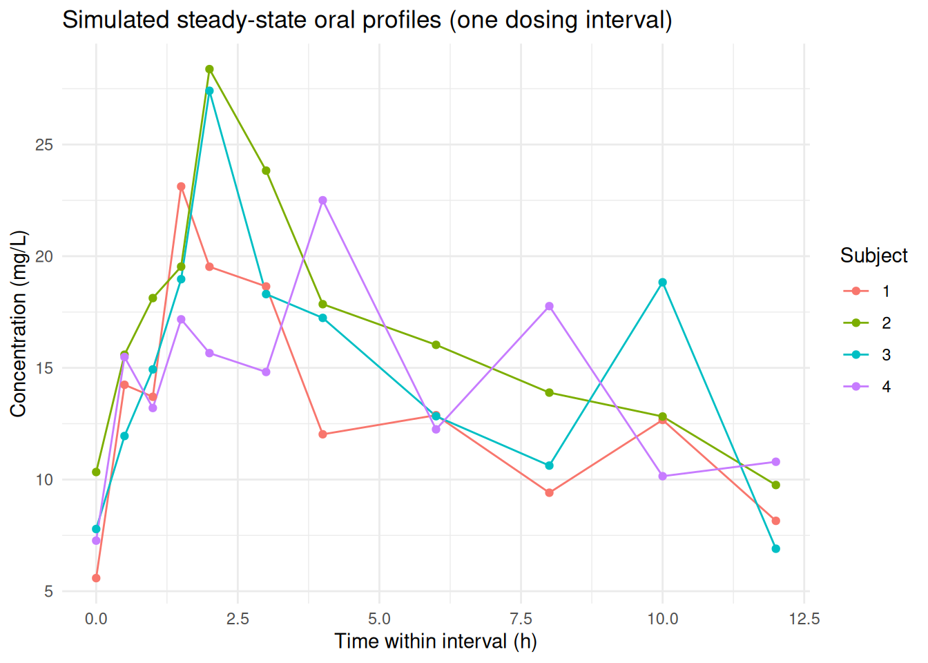
## Synthetic steady-state dataset
We simulate steady-state oral theophylline to demonstrate all parameters. The key is that `start` and `end` define a single dosing interval.
```{r}
set.seed(42)

# Theoph-like PK: Ka=1.5/h, ke=0.08/h, V=30L, dose=400mg
ka <- 1.5; ke <- 0.08; V <- 30; dose <- 400; tau <- 12

# One-compartment oral steady-state: C(t) = [dose/V * ka/(ka-ke)] * [e^(-ke*t)/(1-e^(-ke*tau)) - e^(-ka*t)/(1-e^(-ka*tau))]
C_ss <- function(t, ka, ke, V, dose, tau) {
  A <- (dose / V) * (ka / (ka - ke))
  A * (exp(-ke * t) / (1 - exp(-ke * tau)) - exp(-ka * t) / (1 - exp(-ka * tau)))
}

timepoints <- c(0, 0.5, 1, 1.5, 2, 3, 4, 6, 8, 10, 12)
n_subjects <- 4

d_conc_ss <- expand.grid(Subject = factor(1:n_subjects), time = timepoints) |>
  mutate(
    # Add ~20% log-normal IIV on clearance (ke)
    ke_i  = ke * exp(rnorm(n(), 0, 0.2)),
    conc  = mapply(C_ss, time, ka, ke_i, V, dose, tau) + rnorm(n(), 0, 0.05),
    conc  = pmax(conc, 0)
  ) |>
  select(Subject, time, conc)

d_dose_ss <- data.frame(
  Subject = factor(1:n_subjects),
  dose    = dose,
  time    = 0,
  route   = "extravascular"
)

ggplot(d_conc_ss, aes(x = time, y = conc, group = Subject, colour = Subject)) +
  geom_line() + geom_point() +
  labs(title = "Simulated steady-state oral profiles (one dosing interval)",
       x = "Time within interval (h)", y = "Concentration (mg/L)") +
  theme_minimal()
```
---
## Basic steady-state NCA
For a single dosing interval, set `end = tau`. Parameters like `cav`, `ctrough`, `ptr`, `deg.fluc`, and `swing` all require a finite interval end.
```{r}
o_conc_ss <- PKNCAconc(d_conc_ss, conc ~ time | Subject)
o_dose_ss <- PKNCAdose(d_dose_ss, dose ~ time | Subject, route = "extravascular")
ss_intervals <- data.frame(
  start    = 0,
  end      = tau,
  auclast  = TRUE,
  cmax     = TRUE,
  tmax     = TRUE,
  ctrough  = TRUE,
  cstart   = TRUE,
  cav      = TRUE,
  ptr      = TRUE,
  deg.fluc = TRUE,
  swing    = TRUE
)

o_data_ss <- PKNCAdata(o_conc_ss, o_dose_ss, intervals = ss_intervals)
o_nca_ss  <- pk.nca(o_data_ss)

as.data.frame(o_nca_ss) |>
  filter(PPTESTCD %in% c("auclast", "cmax", "ctrough", "cstart", "cav",
                          "ptr", "deg.fluc", "swing")) |>
  select(Subject, PPTESTCD, PPORRES) |>
  tidyr::pivot_wider(names_from = PPTESTCD, values_from = PPORRES) |>
  arrange(Subject)
```
---
## Parameter reference
### Cstart and Ctrough
`cstart` is the concentration at the **start** of the interval (time = `start`). For steady state this equals the pre-dose trough.
`ctrough` is the concentration at the **end** of the interval (time = `end`). For steady state, `cstart` ≈ `ctrough`.
```{r}
as.data.frame(o_nca_ss) |>
  filter(PPTESTCD %in% c("cstart", "ctrough")) |>
  select(Subject, PPTESTCD, PPORRES) |>
  arrange(Subject, PPTESTCD)
```
### Cav — average concentration
`cav = AUCτ / τ`. Useful for computing clearance at steady state (CL/F = dose / (AUCτ)).
```{r}
as.data.frame(o_nca_ss) |>
  filter(PPTESTCD %in% c("cav", "auclast")) |>
  select(Subject, PPTESTCD, PPORRES) |>
  tidyr::pivot_wider(names_from = PPTESTCD, values_from = PPORRES) |>
  mutate(cav_check = auclast / tau) |>
  arrange(Subject)
```
### PTR, degree of fluctuation, swing
These describe how much concentrations vary within a dosing interval — important for characterizing exposure variability and clinical relevance.
| Parameter | Formula |
|---|---|
| `ptr` | Cmax / Ctrough |
| `deg.fluc` | (Cmax − Cmin) / Cav × 100% |
| `swing` | (Cmax − Cmin) / Cmin × 100% |
```{r}
as.data.frame(o_nca_ss) |>
  filter(PPTESTCD %in% c("ptr", "deg.fluc", "swing")) |>
  select(Subject, PPTESTCD, PPORRES) |>
  tidyr::pivot_wider(names_from = PPTESTCD, values_from = PPORRES) |>
  arrange(Subject)
```
### Ceoi — concentration at end of infusion
For IV infusions, `ceoi` is the concentration at the moment the infusion ends (= `start + duration`). For bolus or oral dosing, it equals `cmax` at the appropriate time.
```{r}
ceoi_interval <- data.frame(
  start  = 0,
  end    = tau,
  ceoi   = TRUE,
  cmax   = TRUE
)

o_nca_ceoi <- pk.nca(PKNCAdata(o_conc_ss, o_dose_ss, intervals = ceoi_interval))

as.data.frame(o_nca_ceoi) |>
  filter(PPTESTCD %in% c("ceoi", "cmax")) |>
  select(Subject, PPTESTCD, PPORRES) |>
  tidyr::pivot_wider(names_from = PPTESTCD, values_from = PPORRES) |>
  arrange(Subject)
```
---
## Multiple dose intervals in one dataset
When data span multiple dose occasions, define one interval row per occasion per group. PKNCA applies each interval independently.
```{r}
# Two dosing intervals: 0-12h and 12-24h
# The t=12 sample belongs to the START of the second interval; exclude it from the first
d_conc_occ1 <- d_conc_ss |> filter(time < 12)   # first interval: 0 to <12
d_conc_occ2 <- d_conc_ss |> mutate(time = time + 12)  # second interval: 12 to 24

d_conc_2dose <- bind_rows(d_conc_occ1, d_conc_occ2)

# Two dose events
d_dose_2dose <- bind_rows(
  d_dose_ss |> mutate(time = 0),
  d_dose_ss |> mutate(time = 12)
)

o_conc_2d <- PKNCAconc(d_conc_2dose, conc ~ time | Subject)
o_dose_2d <- PKNCAdose(d_dose_2dose, dose ~ time | Subject, route = "extravascular")
# One interval per occasion
two_dose_intervals <- data.frame(
  start    = c(0, 12),
  end      = c(12, 24),
  auclast  = TRUE,
  cmax     = TRUE,
  ctrough  = TRUE,
  deg.fluc = TRUE
)

o_nca_2d <- pk.nca(PKNCAdata(o_conc_2d, o_dose_2d, intervals = two_dose_intervals))

as.data.frame(o_nca_2d) |>
  filter(PPTESTCD %in% c("auclast", "cmax", "ctrough")) |>
  select(Subject, start, end, PPTESTCD, PPORRES) |>
  arrange(Subject, start, PPTESTCD)
```
---
## Finding tau automatically: `find.tau()`
When the dosing interval is not known a priori, `find.tau()` estimates it from a numeric vector of dose times. It returns the most common (modal) inter-dose interval.
```{r}
# Dose times for one subject: 0, 12, 24, 36, 48, 60 h
dose_times <- c(0, 12, 24, 36, 48, 60)
find.tau(dose_times)
```
Use the result to construct intervals programmatically:
```{r}
# find.tau() expects one subject's dose times — filter before calling
tau_detected <- find.tau(d_dose_2dose$time[d_dose_2dose$Subject == 1])
cat("Detected tau:", tau_detected, "h\n")
```
---
## Vss at multiple dose (`vss.md.*`)
`vss.md.obs` and `vss.md.pred` are the volume of distribution at steady state using the multiple-dose MRT formula:
$$V_{ss} = CL \times MRT_{md}$$
where MRT_md accounts for the accumulation over repeated dosing.
| Parameter | Meaning |
|---|---|
| `mrt.md.obs` | Multiple-dose MRT (observed Clast) |
| `mrt.md.pred` | Multiple-dose MRT (predicted Clast) |
| `vss.md.obs` | Vss from mrt.md.obs and cl.last |
| `vss.md.pred` | Vss from mrt.md.pred and cl.last |
> **Note:** `vss.md.*` and `mrt.md.*` require the `tau` argument internally but PKNCA 0.12.1 does not correctly resolve it from the interval specification for general use. These parameters work correctly when PKNCA can determine tau from the dosing schedule. Use them in conjunction with explicitly specified tau intervals and verify output against manual calculations.
---
::: {.callout-note icon=false appearance="minimal"}
**pkgdown reference:** [PKNCAconc()](https://humanpred.github.io/pknca/reference/PKNCAconc.html) · [PKNCAdose()](https://humanpred.github.io/pknca/reference/PKNCAdose.html) · [PKNCAdata()](https://humanpred.github.io/pknca/reference/PKNCAdata.html) · [pk.nca()](https://humanpred.github.io/pknca/reference/pk.nca.html) · [find.tau()](https://humanpred.github.io/pknca/reference/find.tau.html)
:::