---
title: "Sparse PK Sampling"
---
```{r setup, include=FALSE}
library(PKNCA)
library(dplyr)
library(ggplot2)
conflicted::conflicts_prefer(dplyr::filter, dplyr::select, .quiet = TRUE)
```
## What is sparse PK?
In **dense PK**, each subject contributes a full concentration-time profile (multiple samples per subject). In **sparse PK**, each subject contributes only one or a few samples, and the population-level profile is reconstructed by pooling across subjects.
Sparse sampling is common in:
- **Preclinical toxicokinetic studies** — serial sacrifice designs where each animal is sampled at only one timepoint
- **Paediatric or special population studies** — where blood volume limits the number of draws per patient
- **Large observational studies** — with opportunistic sampling
PKNCA handles sparse PK by computing a **mean concentration-time profile** across all subjects at each timepoint, then running NCA on that mean profile, along with a standard error estimate from the Nedelman & Jia (1998) method.
---
## Dataset: serial sacrifice design
We construct a synthetic dataset following the Holder et al. (1999) design:
6 nominal timepoints, 3 subjects sampled at each timepoint (18 subjects total, 1 sample each).
```{r}
set.seed(42)

# True PK parameters (oral, 1-compartment)
ka  <- 1.5   # h⁻¹ absorption rate
kel <- 0.25  # h⁻¹ elimination rate
F   <- 1.0
dose <- 100  # mg
V   <- 50    # L

pk_conc <- function(t, ka, kel, dose, V) {
  (dose / V) * (ka / (ka - kel)) * (exp(-kel * t) - exp(-ka * t))
}

timepoints <- c(0, 0.5, 1, 2, 4, 8, 24)  # include t=0 (pre-dose, conc=0)
n_per_time <- 3

d_sparse <- lapply(timepoints, function(t) {
  true_c <- pk_conc(t, ka, kel, dose, V)
  data.frame(
    time    = t,
    conc    = if (t == 0) rep(0, n_per_time)
              else pmax(0, rnorm(n_per_time, mean = true_c, sd = true_c * 0.25)),
    Subject = paste0("S", sprintf("%02d", which(timepoints == t) * 10 + seq_len(n_per_time)))
  )
}) |> bind_rows()

head(d_sparse, 12)
```
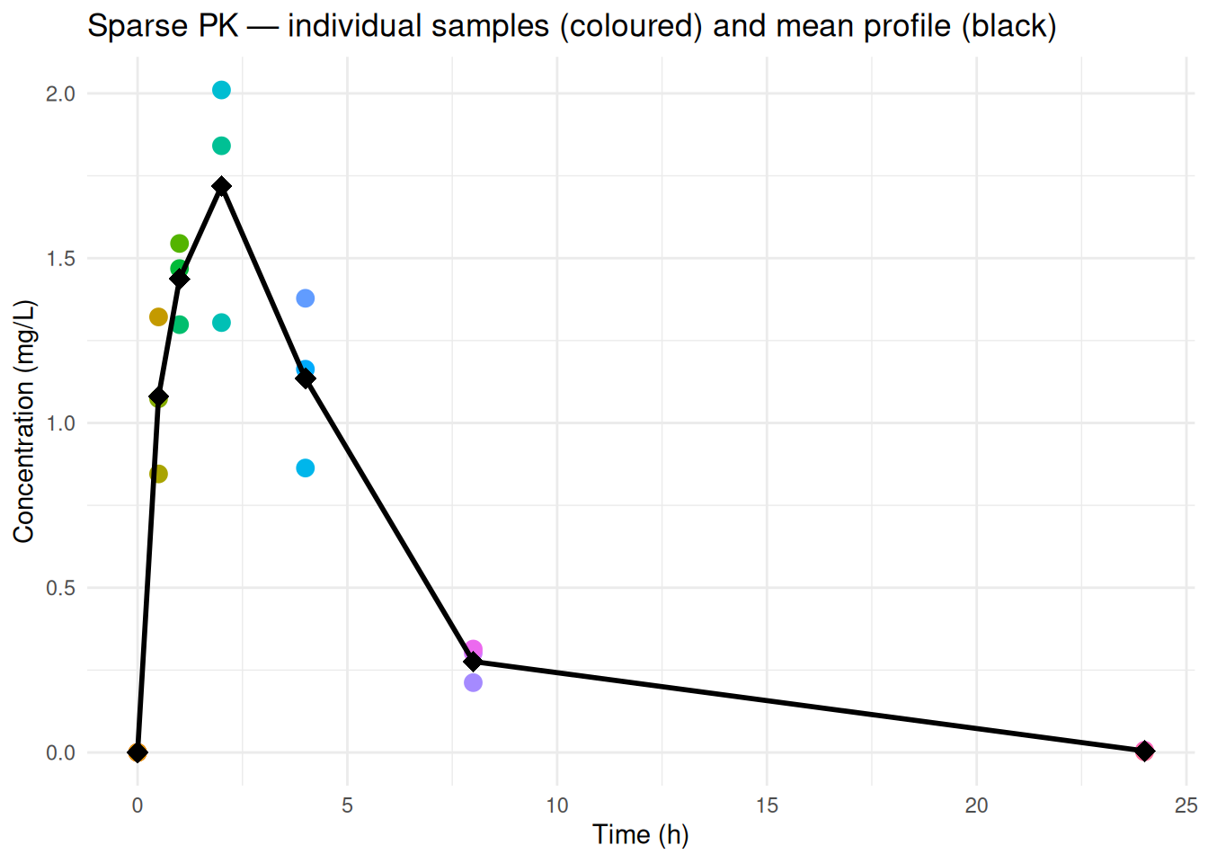
```{r}
ggplot(d_sparse, aes(x = time, y = conc)) +
  geom_point(aes(colour = Subject), size = 3, show.legend = FALSE) +
  stat_summary(fun = mean, geom = "line", linewidth = 1, colour = "black") +
  stat_summary(fun = mean, geom = "point", size = 4, colour = "black", shape = 18) +
  labs(
    title = "Sparse PK — individual samples (coloured) and mean profile (black)",
    x = "Time (h)", y = "Concentration (mg/L)"
  ) +
  theme_minimal()
```
---
## The sparse workflow
The only difference from standard NCA is `sparse = TRUE` in `PKNCAconc()`. Everything else is identical.
```{r}
# Step 1: concentration object — flag as sparse
o_conc <- PKNCAconc(d_sparse, conc ~ time | Subject, sparse = TRUE)

# Step 2: dose object — one row per subject (all received the same dose at t=0)
d_dose <- data.frame(Subject = unique(d_sparse$Subject), dose = dose, time = 0)
o_dose <- PKNCAdose(d_dose, dose ~ time | Subject, route = "extravascular")

# Step 3: data object with sparse interval
o_data <- PKNCAdata(
  o_conc, o_dose,
  intervals = data.frame(
    start          = 0,
    end            = Inf,
    sparse_auclast = TRUE
  )
  # no imputation needed — t=0 pre-dose samples are in the dataset
)

# Step 4: run
o_nca <- pk.nca(o_data)
as.data.frame(o_nca)
```
PKNCA returns three values for sparse AUC:
| Parameter | Meaning |
|---|---|
| `sparse_auclast` | Mean AUC from 0 to last measurable time (Nedelman & Jia method) |
| `sparse_auc_se` | Standard error of the AUC estimate |
| `sparse_auc_df` | Degrees of freedom for confidence interval construction |
---
## How PKNCA computes sparse AUC
1. At each timepoint, compute the **mean concentration** across subjects (pooling all subjects sampled at that time)
2. Apply the **lin up / log down** trapezoidal rule to the mean profile to get AUClast
3. Estimate **variance** using the Nedelman & Jia (1998) formula, accounting for the covariance between AUC trapezoids via the Holder (2001) method
4. Return AUClast ± SE and degrees of freedom
```{r}
# Inspect the mean profile PKNCA uses internally
mean_profile <- d_sparse |>
  group_by(time) |>
  summarise(mean_conc = mean(conc), n = n(), se = sd(conc) / sqrt(n()), .groups = "drop")

mean_profile
```
---
## BLQ handling in sparse PK
`sparse = TRUE` affects how BLQ values (coded as 0) are treated at each timepoint before averaging. The default BLQ treatment is controlled by `PKNCA.options("conc.blq")` and applies **before** the mean is computed.
Available mean methods (controlled internally):
- **`"arithmetic mean"`** — simple mean of all values including BLQs as 0
- **`"arithmetic mean, <=50% BLQ"`** — if **strictly more than 50%** of subjects at a timepoint are BLQ, the mean concentration at that timepoint is set to 0 (at exactly 50% BLQ the mean is not zeroed)
The second method is conservative: timepoints with majority-BLQ results don't pull the mean above zero.
---
## Serial sacrifice vs. repeated sampling
```{r}
# Serial sacrifice: each subject contributes EXACTLY 1 sample
d_serial <- d_sparse  # our example above — each subject is at one timepoint only

# Mixed design: some subjects contribute multiple samples
# (PKNCA handles this too — subjects can appear at multiple times)
d_mixed <- bind_rows(
  d_sparse,
  data.frame(time = 4, conc = 0.8, Subject = "S11"),  # S11 sampled at 2 times
  data.frame(time = 8, conc = 0.3, Subject = "S11")
)

d_dose_mixed <- data.frame(Subject = unique(d_mixed$Subject), dose = dose, time = 0)
o_dose_mixed  <- PKNCAdose(d_dose_mixed, dose ~ time | Subject, route = "extravascular")
o_conc_mixed  <- PKNCAconc(d_mixed, conc ~ time | Subject, sparse = TRUE)
o_data_mixed  <- PKNCAdata(
  o_conc_mixed, o_dose_mixed,
  intervals = data.frame(start = 0, end = Inf, sparse_auclast = TRUE)
)
o_nca_mixed <- pk.nca(o_data_mixed)
# Note: degrees of freedom (sparse_auc_df) cannot be calculated
# when any subject contributes multiple samples — a current PKNCA limitation
as.data.frame(o_nca_mixed)
```
> **Limitation:** `sparse_auc_df` is `NA` when any subject contributes more than one sample per interval. This is a known current limitation of the Nedelman & Jia variance estimation in PKNCA.
---
## Constructing a confidence interval
With AUC, SE, and df you can construct a t-based confidence interval:
```{r}
res <- as.data.frame(o_nca) |>
  tidyr::pivot_wider(names_from = PPTESTCD, values_from = PPORRES)

auc <- res$sparse_auclast
se  <- res$sparse_auc_se
df  <- res$sparse_auc_df

if (!is.na(df) && !is.na(se)) {
  ci_lo <- auc - qt(0.975, df) * se
  ci_hi <- auc + qt(0.975, df) * se
  cat(sprintf("AUClast = %.2f  95%% CI: [%.2f, %.2f]\n", auc, ci_lo, ci_hi))
} else {
  cat(sprintf("AUClast = %.2f  SE = %.2f  (df unavailable for CI)\n", auc, se))
}
```
---
## Key differences from dense NCA
| Aspect | Dense PK | Sparse PK |
|---|---|---|
| `PKNCAconc` flag | `sparse = FALSE` (default) | `sparse = TRUE` |
| Profile per subject | Full individual profile | 1–few samples only |
| NCA run on | Each subject's own profile | Pooled mean profile |
| Result | One row per subject per parameter | One row per parameter (population level) |
| Half-life | ✓ (per subject) | ✗ (not available) |
| AUClast | ✓ | ✓ (`sparse_auclast`) |
| SE of AUC | ✗ | ✓ (`sparse_auc_se`) |
| Interval col name | `auclast` | `sparse_auclast` |
---
## Available sparse parameters
```{r}
cols <- get.interval.cols()
sparse_params <- Filter(function(x) isTRUE(x$sparse), cols)
data.frame(
  parameter   = names(sparse_params),
  description = sapply(sparse_params, `[[`, "desc")
) |> knitr::kable()
```
---
## Sparse AUMC and derived parameters (≥ 0.12.2)
PKNCA ≥ 0.12.2 adds sparse AUMC (area under the first-moment curve) and five new derived parameters, enabling MRT, clearance, and volume estimation from sparse data.
### Sparse AUMC
| Parameter | Description |
|---|---|
| `sparse_aumclast` | AUMC from the pooled mean sparse profile (0 → last measurable) |
| `sparse_aumc_se` | Standard error of the sparse AUMC estimate |
| `sparse_aumc_df` | Degrees of freedom for the AUMC variance estimate |
Requesting `sparse_aumclast = TRUE` automatically computes `sparse_auclast`, `sparse_auc_se`, `sparse_auc_df`, `sparse_aumc_se`, and `sparse_aumc_df` as dependencies.
```{r}
sparse_aumc_interval <- data.frame(
  start           = 0,
  end             = Inf,
  sparse_aumclast = TRUE   # AUC and SE are computed automatically as dependencies
)

o_nca_sparse_aumc <- pk.nca(PKNCAdata(o_conc, o_dose, intervals = sparse_aumc_interval))

as.data.frame(o_nca_sparse_aumc) |>
  select(PPTESTCD, PPORRES)
```
### Sparse-derived PK parameters
Once sparse AUC and AUMC are available, PKNCA can compute additional population-level parameters:
| Parameter | Description |
|---|---|
| `mrt.sparse.last` | Mean residence time from sparse sampling |
| `cl.sparse.last` | Clearance: dose / sparse AUClast |
| `kel.sparse.last` | Elimination rate constant: 1 / MRT_sparse |
| `vss.sparse.last` | Steady-state volume of distribution from sparse sampling |
| `vz.sparse.last` | Terminal volume of distribution from sparse sampling |
```{r}
sparse_full_interval <- data.frame(
  start           = 0,
  end             = Inf,
  sparse_aumclast = TRUE,   # also pulls in sparse_auclast, SE, df
  mrt.sparse.last = TRUE,
  cl.sparse.last  = TRUE,
  kel.sparse.last = TRUE
)

o_nca_sparse_full <- pk.nca(PKNCAdata(o_conc, o_dose, intervals = sparse_full_interval))

as.data.frame(o_nca_sparse_full) |>
  filter(PPTESTCD %in% c("sparse_auclast", "sparse_aumclast",
                          "mrt.sparse.last", "cl.sparse.last", "kel.sparse.last")) |>
  select(PPTESTCD, PPORRES)
```
> `vss.sparse.last` and `vz.sparse.last` require a terminal elimination estimate (λz) which cannot be derived from the pooled mean sparse profile alone; they return `NA` unless additional terminal-phase information is available.
---
::: {.callout-note icon=false appearance="minimal"}
**pkgdown reference:** [PKNCAconc()](https://humanpred.github.io/pknca/reference/PKNCAconc.html) · [PKNCAdose()](https://humanpred.github.io/pknca/reference/PKNCAdose.html) · [PKNCAdata()](https://humanpred.github.io/pknca/reference/PKNCAdata.html) · [pk.nca()](https://humanpred.github.io/pknca/reference/pk.nca.html) · [get.interval.cols()](https://humanpred.github.io/pknca/reference/get.interval.cols.html)
:::