---
title: "Post-Processing Results"
---
```{r setup, include=FALSE}
library(PKNCA)
library(dplyr)
library(ggplot2)
conflicted::conflicts_prefer(dplyr::filter, dplyr::select, .quiet = TRUE)
d_conc <- as.data.frame(Theoph) |> rename(time = Time, subject = Subject)
d_dose <- Theoph |> as.data.frame() |>
group_by(Subject) |>
summarise(dose = Dose[1] * Wt[1], weight = Wt[1], .groups = "drop") |>
rename(subject = Subject) |>
mutate(time = 0)
o_conc <- PKNCAconc(d_conc, conc ~ time | subject)
o_dose <- PKNCAdose(d_dose, dose ~ time | subject, route = "extravascular")
o_data <- PKNCAdata(o_conc, o_dose, intervals = data.frame(
start = 0, end = Inf,
auclast = TRUE, aucinf.obs = TRUE, cmax = TRUE,
half.life = TRUE, span.ratio = TRUE, adj.r.squared = TRUE,
aucpext.obs = TRUE
))
o_nca <- pk.nca(o_data)
```
## Why post-process?
After `pk.nca()` you may need to:
1. **Exclude** specific results that failed QC (poor half-life fit, protocol deviation)
2. **Normalize** parameters by dose (built-in `.dn` variants)
3. **Summarize** with custom statistics, respecting exclusions
All of this operates on the `PKNCAresults` object without rerunning the analysis.
---
## Excluding results
### Manual exclusion with `exclude()`
`exclude()` takes your results object plus a `reason` string and either a logical `mask` or a rule `FUN`. Excluding a parameter automatically excludes all downstream parameters that depend on it.
```{r}
# Exclude subject 3's half-life manually (e.g., failed QC review)
o_nca_excl <- exclude(
  o_nca,
  reason = "half-life failed manual QC",
  mask   = as.data.frame(o_nca)$subject == "3" &
           as.data.frame(o_nca)$PPTESTCD == "half.life"
)

# Exclusion propagates to aucinf.obs (depends on lambda.z which depends on half.life)
as.data.frame(o_nca_excl) |>
  filter(subject == "3", !is.na(exclude)) |>
  select(subject, PPTESTCD, PPORRES, exclude)
```
### Rule-based exclusion functions
PKNCA provides ready-made rule functions to pass to `exclude(FUN=...)`:
| Function | Excludes when... |
|---|---|
| `exclude_nca_span.ratio(min)` | span.ratio < min |
| `exclude_nca_min.hl.r.squared(min)` | half-life unadjusted R² < min |
| `exclude_nca_min.hl.adj.r.squared(min)` | half-life adjusted R² < min (stricter, accounts for number of points) |
| `exclude_nca_max.aucinf.pext(max)` | %AUCextrap > max |
| `exclude_nca_tmax_0()` | Tmax = 0 (no absorption observed) |
| `exclude_nca_tmax_early()` | Tmax is at first timepoint |
| `exclude_nca_count_conc_measured(min)` | too few measured concentrations |
| `exclude_nca_by_param(params)` | exclude specific parameters by name |
```{r}
# Exclude half-lives where span ratio < 2
o_nca_span <- exclude(
  o_nca,
  reason = "span.ratio < 2",
  FUN    = exclude_nca_span.ratio(2)
)
as.data.frame(o_nca_span) |>
  filter(PPTESTCD == "half.life") |>
  select(subject, PPORRES, exclude) |>
  arrange(subject)
```
```{r}
# Chain multiple exclusion rules
o_nca_multi <- o_nca |>
  exclude(reason = "span.ratio < 2",    FUN = exclude_nca_span.ratio(2)) |>
  exclude(reason = "%AUCextrap > 20%",  FUN = exclude_nca_max.aucinf.pext(20))

as.data.frame(o_nca_multi) |>
  filter(!is.na(exclude)) |>
  select(subject, PPTESTCD, exclude) |>
  arrange(subject, PPTESTCD)
```
### Exclusions are respected in summary
```{r}
summary(o_nca_span)
```
---
## Dose-normalized parameters
PKNCA has built-in dose-normalized variants for several parameters. Request them in the interval — they are automatically computed as `parameter / dose`.
All available dose-normalized parameters (retrieved dynamically from registry):
```{r}
cols <- get.interval.cols()
dn_params <- names(cols)[endsWith(names(cols), ".dn")]
data.frame(
  parameter       = dn_params,
  description     = sapply(cols[dn_params], function(x) x$desc),
  normalized_from = sub("\\.dn$", "", dn_params)
) |> knitr::kable()
```
Each `.dn` parameter is computed as `parameter / dose` where `dose` is the dose from the `PKNCAdose` object for that interval. In PKNCA ≥ 0.12.2 this includes renal clearance variants (`clr.last.dn`, `clr.obs.dn`, `clr.pred.dn`).
### Custom normalization with `normalize()` (≥ 0.12.2)
For normalization by columns other than dose (e.g., body weight, body surface area), PKNCA 0.12.2 adds `normalize()`. You supply a `norm_table` data frame containing the grouping columns, a `normalization` value, and a `unit` for each group:
```{r}
# Normalize AUClast and Cmax by body weight
norm_tbl <- as.data.frame(Theoph) |>
  group_by(Subject) |>
  summarise(normalization = Wt[1], unit = "kg", .groups = "drop") |>
  rename(subject = Subject)

df_results <- as.data.frame(o_nca)
df_bw_norm <- normalize(
  df_results,
  norm_table  = norm_tbl,
  parameters  = c("auclast", "cmax"),
  suffix      = ".bw"
)

df_bw_norm |>
  select(subject, PPTESTCD, PPORRES) |>
  arrange(subject, PPTESTCD) |>
  head(8)
```
> `normalize()` **replaces** the specified parameters in the result — `auclast` becomes `auclast.bw`, `cmax` becomes `cmax.bw`. To keep both original and normalized values, run `normalize()` on a copy and then `bind_rows()`.
`normalize_by_col()` is the low-level variant that pulls normalization values from a column already present in the `PKNCAconc` data frame, rather than from a separate table.
```{r}
dn_interval <- data.frame(
  start           = 0,
  end             = Inf,
  auclast         = TRUE,
  auclast.dn      = TRUE,   # AUClast / dose
  aucinf.obs      = TRUE,
  aucinf.obs.dn   = TRUE,   # AUCinf.obs / dose
  aucinf.pred.dn  = TRUE,   # AUCinf.pred / dose
  cmax            = TRUE,
  cmax.dn         = TRUE,   # Cmax / dose
  cmin.dn         = TRUE,   # Cmin / dose
  aumclast.dn     = TRUE,   # AUMClast / dose
  clast.obs.dn    = TRUE,   # Clast.obs / dose
  cav.dn          = TRUE,   # Cav / dose
  half.life       = TRUE    # needed for aucinf.pred
)

o_nca_dn <- pk.nca(PKNCAdata(o_conc, o_dose, intervals = dn_interval))

as.data.frame(o_nca_dn) |>
  filter(PPTESTCD %in% c("auclast", "auclast.dn", "cmax", "cmax.dn",
                          "aucinf.obs", "aucinf.obs.dn")) |>
  select(subject, PPTESTCD, PPORRES) |>
  tidyr::pivot_wider(names_from = PPTESTCD, values_from = PPORRES) |>
  arrange(subject)
```
---
## Extracting results
`as.data.frame()` returns the full tidy result including excluded rows:
```{r}
df <- as.data.frame(o_nca)

# Columns:
# subject    — group identifier
# start/end  — interval boundaries
# PPTESTCD   — parameter code
# PPORRES    — numeric result
# exclude    — NA if valid; character reason if excluded

df |>
  filter(PPTESTCD == "auclast") |>
  select(subject, PPORRES, exclude) |>
  arrange(subject)
```
---
## Custom summary statistics
`PKNCA.set.summary()` controls how each parameter is presented in `summary()`.
```{r}
# Arithmetic mean ± SD for AUClast
PKNCA.set.summary(
  "auclast",
  description = "mean ± SD",
  point  = mean,
  spread = sd
)

# Median [min, max] for Tmax
# spread must return a 2-element numeric vector
PKNCA.set.summary(
  "tmax",
  description = "median [min, max]",
  point  = median,
  spread = function(x) c(min(x), max(x))
)

summary(o_nca)
```
Restore to default (geometric mean ± geometric CV%):
```{r}
PKNCA.set.summary(
  "auclast",
  description = "geometric mean [geometric CV%]",
  point  = PKNCA::geomean,
  spread = PKNCA::geocv
)

PKNCA.set.summary(
  "tmax",
  description = "median [min, max]",
  point  = median,
  spread = function(x) c(min(x), max(x))
)
```
---
## Business summary helpers
PKNCA exports the full set of `business.*` summary functions. These are used internally by `PKNCA.set.summary()` and are also available directly for custom reporting pipelines.
| Function | Returns | Description |
|---|---|---|
| `business.geomean(x)` | scalar | Geometric mean: exp(mean(log(x))) |
| `business.geocv(x)` | scalar | Geometric CV%: sqrt(exp(var(log(x)))−1) × 100 |
| `business.mean(x)` | scalar | Arithmetic mean |
| `business.sd(x)` | scalar | Standard deviation |
| `business.cv(x)` | scalar | Coefficient of variation %: sd/mean × 100 |
| `business.median(x)` | scalar | Median |
| `business.min(x)` | scalar | Minimum |
| `business.max(x)` | scalar | Maximum |
| `business.range(x)` | length-2 vector | c(min, max) |
```{r}
x <- c(10.2, 11.8, 9.6, 12.1, 10.5)
data.frame(
  statistic = c("geomean", "geocv", "mean", "sd", "cv%", "median", "min", "max"),
  value = c(
    business.geomean(x), business.geocv(x),
    business.mean(x),    business.sd(x),    business.cv(x),
    business.median(x),  business.min(x),   business.max(x)
  )
)
```
Use these as `point` and `spread` arguments to `PKNCA.set.summary()`:
```{r}
# Arithmetic mean ± CV% for Cmax
PKNCA.set.summary(
  "cmax",
  description = "mean [CV%]",
  point  = business.mean,
  spread = business.cv
)
```
---
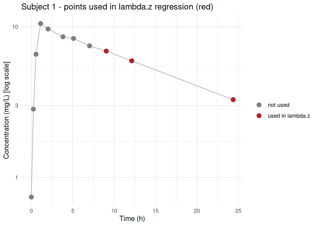
## Inspecting the terminal regression window
`get_halflife_points()` returns a logical vector aligned with the original concentration data — `TRUE` if that observation was used in the λz regression, `FALSE` if it was available but excluded, `NA` if half-life was not computed for that interval. In PKNCA ≥ 0.12.2 it also accepts a `PKNCAdata` object directly and handles `start ≠ 0` intervals correctly.
```{r}
d_conc_pp <- as.data.frame(Theoph) |> rename(time = Time, subject = Subject)
d_dose_pp <- Theoph |> as.data.frame() |>
  group_by(Subject) |>
  summarise(dose = Dose[1] * Wt[1], .groups = "drop") |>
  rename(subject = Subject) |>
  mutate(time = 0)

o_conc_pp <- PKNCAconc(d_conc_pp, conc ~ time | subject)
o_dose_pp <- PKNCAdose(d_dose_pp, dose ~ time | subject, route = "extravascular")
o_nca_pp  <- pk.nca(PKNCAdata(o_conc_pp, o_dose_pp,
                               intervals = data.frame(start = 0, end = Inf, half.life = TRUE)))

# Logical vector (TRUE = used in lambda.z fit)
hl_used <- get_halflife_points(o_nca_pp)
table(hl_used, useNA = "always")
```
```{r}
# Attach to concentration data for plotting
d_conc_annotated <- d_conc_pp |> mutate(in_lambda_z = hl_used)
subj1_conc <- d_conc_annotated |> filter(subject == "1")

ggplot(subj1_conc, aes(x = time, y = conc, colour = in_lambda_z)) +
  geom_line(colour = "grey70") +
  geom_point(size = 3) +
  scale_colour_manual(values = c("FALSE" = "grey50", "TRUE" = "firebrick"),
                      labels = c("not used", "used in lambda.z"), name = NULL,
                      na.value = "grey80") +
  scale_y_log10() +
  labs(title = "Subject 1 - points used in lambda.z regression (red)",
       x = "Time (h)", y = "Concentration (mg/L) [log scale]") +
  theme_minimal()
```
---
## Imputation methods
PKNCA supports pre-dose and post-dose concentration imputation strategies, controlled by the `impute` argument to `PKNCAdata()` or by columns in the concentration data.
Built-in imputation strategies:
| Strategy | When it applies | What it does |
|---|---|---|
| `"start_conc0"` | Interval start before first measured time | Adds conc = 0 at the interval start time |
| `"start_predose"` | Interval start before first measured time | Uses the last pre-dose (pre-interval) concentration |
| `"start_cmin"` | Interval start before first measured time | Uses the minimum observed concentration in the interval |
All three strategies are implemented as exported functions — `PKNCA_impute_method_start_conc0()`, `PKNCA_impute_method_start_predose()`, `PKNCA_impute_method_start_cmin()` — and can also be referenced by their string names.
```{r}
# Theoph subject 1 starts at t=0 — simulate a dataset with no t=0 sample
d_conc_imp <- d_conc_pp |> filter(subject == "1", time > 0)
o_conc_imp <- PKNCAconc(d_conc_imp, conc ~ time | subject)
o_dose_imp <- PKNCAdose(
  d_dose_pp |> filter(subject == "1"),
  dose ~ time | subject,
  route = "extravascular"
)

ivl <- data.frame(start = 0, end = Inf, auclast = TRUE)

r_conc0   <- pk.nca(PKNCAdata(o_conc_imp, o_dose_imp, intervals = ivl, impute = "start_conc0"))
r_cmin    <- pk.nca(PKNCAdata(o_conc_imp, o_dose_imp, intervals = ivl, impute = "start_cmin"))

# start_predose uses last pre-dose conc; with no pre-dose sample it returns NA
r_predose <- pk.nca(PKNCAdata(o_conc_imp, o_dose_imp, intervals = ivl, impute = "start_predose"))
bind_rows(
  as.data.frame(r_conc0)   |> filter(PPTESTCD == "auclast") |> mutate(strategy = "start_conc0"),
  as.data.frame(r_cmin)    |> filter(PPTESTCD == "auclast") |> mutate(strategy = "start_cmin"),
  as.data.frame(r_predose) |> filter(PPTESTCD == "auclast") |> mutate(strategy = "start_predose")
) |>
  select(strategy, PPTESTCD, PPORRES)
```
> **Choosing a strategy:** `start_conc0` is appropriate for drugs fully eliminated between doses or for the first dose. `start_predose` is appropriate when a pre-dose (trough) sample was collected. `start_cmin` is a conservative option when no pre-dose sample was collected and a zero is not pharmacologically appropriate.
---
::: {.callout-note icon=false appearance="minimal"}
**pkgdown reference:** [PKNCAconc()](https://humanpred.github.io/pknca/reference/PKNCAconc.html) · [PKNCAdose()](https://humanpred.github.io/pknca/reference/PKNCAdose.html) · [PKNCAdata()](https://humanpred.github.io/pknca/reference/PKNCAdata.html) · [pk.nca()](https://humanpred.github.io/pknca/reference/pk.nca.html) · [exclude()](https://humanpred.github.io/pknca/reference/exclude.html) · [normalize()](https://humanpred.github.io/pknca/reference/normalize.html) · [normalize_by_col()](https://humanpred.github.io/pknca/reference/normalize_by_col.html) · [get_halflife_points()](https://humanpred.github.io/pknca/reference/get_halflife_points.html) · [PKNCA.set.summary()](https://humanpred.github.io/pknca/reference/PKNCA.set.summary.html)
:::