---
title: "Dose-Aware Interpolation and Extrapolation"
---
```{r setup, include=FALSE}
library(PKNCA)
library(dplyr)
library(ggplot2)
conflicted::conflicts_prefer(dplyr::filter, dplyr::select, .quiet = TRUE)
```
## Why dose timing matters for interpolation
Standard concentration interpolation (e.g., `interp.extrap.conc()`) assumes a smooth concentration-time curve with no discontinuities. But when a dose is given **at** or **near** the interpolation target time, the correct value depends critically on whether you are asking about the concentration *before* or *after* that dose event.
**`interp.extrap.conc.dose()`** is the dose-aware version. It accounts for:
- Whether the route is intravascular (bolus causes instantaneous jump) or extravascular (no instantaneous change)
- Whether you want the concentration before (`out.after = FALSE`) or after (`out.after = TRUE`) the dose
- Whether the dose is an infusion with a finite duration
---
## The key argument: `out.after`
| `out.after` | Meaning |
|---|---|
| `FALSE` (default) | Return the concentration just **before** the dose event |
| `TRUE` | Return the concentration just **after** the dose event |
For extravascular doses, there is no instantaneous concentration change at the dose time, so `out.after` only affects the behaviour right at the dose time itself.
For IV bolus, the dose causes an instantaneous jump, so the before/after distinction is pharmacologically meaningful.
---
## Shared example data
```{r}
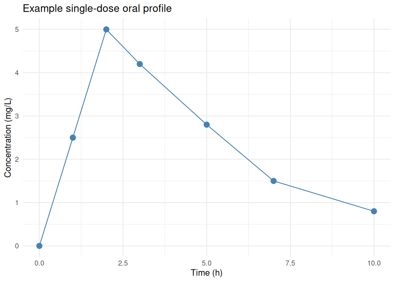
# Single-dose oral profile (absorption + elimination)
conc <- c(0.0, 2.5, 5.0, 4.2, 2.8, 1.5, 0.8)
time <- c(0,   1,   2,   3,   5,   7,   10 )

d <- data.frame(time = time, conc = conc)

ggplot(d, aes(x = time, y = conc)) +
  geom_line(colour = "steelblue") +
  geom_point(size = 3, colour = "steelblue") +
  labs(title = "Example single-dose oral profile",
       x = "Time (h)", y = "Concentration (mg/L)") +
  theme_minimal()
```
---
## Basic interpolation (no dose at target time)
When the target time is **between** observed samples and does not coincide with a dose, the result equals standard log-linear interpolation.
```{r}
# t = 4h falls between t=3 and t=5
interp.extrap.conc.dose(
  conc       = conc,
  time       = time,
  time.dose  = 0,          # dose was given at t=0
  route.dose = "extravascular",
  time.out   = 4
)
```
Compare to dose-unaware interpolation:
```{r}
interp.extrap.conc(conc = conc, time = time, time.out = 4)
```
They agree when no dose occurs at the target time.
---
## At the dose time: oral (extravascular)
For an oral dose, concentration does not change instantaneously at the dose time — absorption is gradual. So `out.after` does not change the interpolated value at the dose time itself.
```{r}
# Oral: t=0, before dose
interp.extrap.conc.dose(
  conc       = conc, time = time,
  time.dose  = 0, route.dose = "extravascular",
  time.out   = 0, out.after  = FALSE
)
```
```{r}
# Oral: t=0, after dose (same — no jump)
interp.extrap.conc.dose(
  conc       = conc, time = time,
  time.dose  = 0, route.dose = "extravascular",
  time.out   = 0, out.after  = TRUE
)
```
---
## At the dose time: IV bolus (intravascular)
For an IV bolus, the dose causes an instantaneous concentration jump. `out.after = FALSE` returns the pre-dose (trough) concentration; `out.after = TRUE` returns the post-dose concentration.
```{r}
# IV profile: C0 = 10 after dose, declines monoexponentially
conc_iv <- c(10,  8,  6,  4,  2.5, 1.5)
time_iv <- c(0,   1,  2,  4,  6,   9  )

# Before second dose at t=6 — return the trough
interp.extrap.conc.dose(
  conc       = conc_iv, time = time_iv,
  time.dose  = 0, route.dose = "intravascular",
  time.out   = 6, out.after  = FALSE
)
```
---
## Multiple dose times
Provide a vector to `time.dose` when multiple doses were given during the sampling window.
```{r}
# Oral doses at t=0 and t=6
conc_md <- c(0, 2.5, 5.0, 4.2, 2.8, 4.5, 6.0, 5.1, 3.5, 2.0)
time_md <- c(0, 1,   2,   3,   5,   6,   7,   8,   10,  12 )

# Concentration just before the second dose at t=6
interp.extrap.conc.dose(
  conc       = conc_md, time = time_md,
  time.dose  = c(0, 6), route.dose = "extravascular",
  time.out   = 6, out.after = FALSE
)
```
```{r}
# Concentration just after the second dose at t=6
interp.extrap.conc.dose(
  conc       = conc_md, time = time_md,
  time.dose  = c(0, 6), route.dose = "extravascular",
  time.out   = 6, out.after = TRUE
)
```
For extravascular doses, before and after are the same (no instantaneous jump).
---
## IV infusion: dose duration
For IV infusions, supply `duration.dose` (the infusion duration in the same time units).
```{r}
# 30-minute (0.5h) infusion starting at t=0
conc_inf <- c(0, 3,  5,  4.5, 3,  2,  1  )
time_inf <- c(0, 0.25, 0.5, 1, 2, 4, 8  )

# At end of infusion (t=0.5): concentration is the measured peak
interp.extrap.conc.dose(
  conc          = conc_inf, time = time_inf,
  time.dose     = 0,
  route.dose    = "intravascular",
  duration.dose = 0.5,
  time.out      = 0.5, out.after = FALSE
)
```
---
## How PKNCA uses `interp.extrap.conc.dose()` internally
PKNCA calls this function automatically whenever an interval boundary (the `start` or `end` of an interval in your intervals data frame) falls at a dose time. You normally never call it directly.
Understanding its behaviour helps diagnose unusual NCA results when dosing and sampling times coincide — for example, when `start = tau` (the trough time) is also the time of the next dose.
---
## Argument reference
| Argument | Required | Meaning |
|---|---|---|
| `conc` | Yes | Observed concentrations |
| `time` | Yes | Observation times (same units as `time.dose`) |
| `time.dose` | Yes | Time(s) at which doses were given |
| `route.dose` | Yes | `"extravascular"` or `"intravascular"` |
| `duration.dose` | No | Infusion duration (NA = bolus) |
| `time.out` | Yes | Target time at which to interpolate/extrapolate |
| `out.after` | No (default `FALSE`) | `FALSE` = before dose; `TRUE` = after dose |
| `options` | No | PKNCA options list (controls AUC method / interpolation rule) |
---
::: {.callout-note icon=false appearance="minimal"}
**pkgdown reference:** [interp.extrap.conc.dose()](https://humanpred.github.io/pknca/reference/interp.extrap.conc.dose.html) · [interp.extrap.conc()](https://humanpred.github.io/pknca/reference/interp.extrap.conc.html)
:::