Selection of Calculation Intervals
Bill Denney
Source:vignettes/v03-selection-of-calculation-intervals.Rmd
v03-selection-of-calculation-intervals.RmdIntroduction
PKNCA considers two types of data grouping within data sets: the group and the interval. A group typically identifies a single subject given a single intervention type (a “treatment”) with a single analyte. An interval subsets a group by times within the group, and primary noncompartmental analysis (NCA) calculations are performed within an interval.
As a concrete example, consider the figure below shows the concentration-time profile of a study subject in a multiple-dose study. The group is all points in the figure, and the interval for the last day (144 to 168 hr) is the area with blue shading.
## Formula for concentration:
##  conc ~ time | treatment + ID
## Data are dense PK.
## With 1 subjects defined in the 'ID' column.
## Nominal time column is not specified.
##
## First 6 rows of concentration data:
##    study treatment ID time      conc   analyte exclude
##  Study 1     Trt 1  1    0 0.0000000 Analyte 1    <NA>
##  Study 1     Trt 1  1    1 0.6140526 Analyte 1    <NA>
##  Study 1     Trt 1  1    2 0.8100022 Analyte 1    <NA>
##  Study 1     Trt 1  1    4 0.8425422 Analyte 1    <NA>
##  Study 1     Trt 1  1    6 0.7771994 Analyte 1    <NA>
##  Study 1     Trt 1  1    8 0.7052469 Analyte 1    <NA>
# Plot the concentration-time data and the interval
ggplot(d_conc_multi, aes(x=time, y=conc)) +
  geom_ribbon(data=d_conc_multi[d_conc_multi$time >= 144,],
              aes(ymax=conc, ymin=0),
              fill="skyblue") +
  geom_point() + geom_line() +
  scale_x_continuous(breaks=seq(0, 168, by=12)) +
  scale_y_continuous(limits=c(0, NA)) +
  labs(x="Time Since First Dose (hr)",
       y="Concentration\n(arbitrary units)")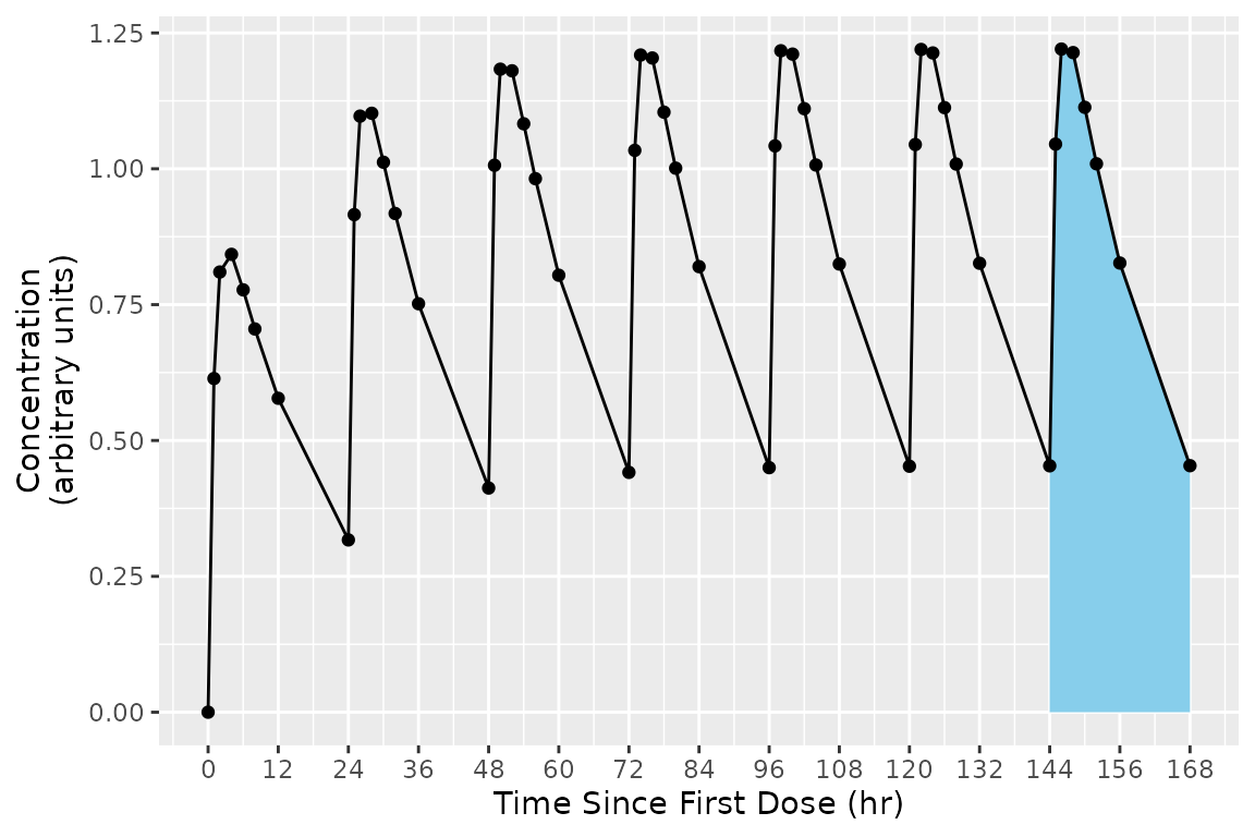
intervals_manual <- data.frame(start=144, end=168, auclast=TRUE)
knitr::kable(intervals_manual)| start | end | auclast |
|---|---|---|
| 144 | 168 | TRUE |
d_conc_multi_obj <- PKNCAconc(d_conc_multi, conc~time|treatment+ID)
PKNCAdata(d_conc_multi_obj, intervals=intervals_manual)
## Formula for concentration:
## conc ~ time | treatment + ID
## Data are dense PK.
## With 1 subjects defined in the 'ID' column.
## Nominal time column is not specified.
##
## First 6 rows of concentration data:
## treatment ID conc time exclude
## Trt 1 1 0.0000000 0 <NA>
## Trt 1 1 0.6140526 1 <NA>
## Trt 1 1 0.8100022 2 <NA>
## Trt 1 1 0.8425422 4 <NA>
## Trt 1 1 0.7771994 6 <NA>
## Trt 1 1 0.7052469 8 <NA>
## No dosing information.
##
## With 1 rows of interval specifications.
## No options are set differently than default.Group Matching
Group matching occurs by matching all overlapping column names
between the groups and the interval data.frame. (Note that grouping
columns cannot be the word start, end, or
share a name with an NCA parameter.)
Selecting the Subjects for an Interval
The groups for an interval prepare for summarization. Typically the groups will take a structure similar to the preferred summarization structure with groups nested in the logical method for summary. As an example, the group structure may be: study, treatment, day, analyte, and subject. The grouping names for an interval must be the same as or a subset of the grouping names used for the concentration data.
As the matching occurs with all available columns, the grouping columns names are only required to the level of specificity for the calculations desired. As an example, if you want AUCinf,obs in subjects who received single doses and AUClast on days 1 (0 to 24 hours) and 10 (216 to 240 hours) in subjects who received multiple doses, with treatment defined as “Drug 1 Single” or “Drug 1 Multiple”, the intervals could be defined as below.
intervals_manual <-
  data.frame(
    treatment=c("Drug 1 Single", "Drug 1 Multiple", "Drug 1 Multiple"),
    start=c(0, 0, 216),
    end=c(Inf, 24, 240),
    aucinf.obs=c(TRUE, FALSE, FALSE),
    auclast=c(FALSE, TRUE, TRUE)
  )
knitr::kable(intervals_manual)| treatment | start | end | aucinf.obs | auclast |
|---|---|---|---|---|
| Drug 1 Single | 0 | Inf | TRUE | FALSE |
| Drug 1 Multiple | 0 | 24 | FALSE | TRUE |
| Drug 1 Multiple | 216 | 240 | FALSE | TRUE |
Intervals
Intervals are defined by data.frames with one row per
interval, zero or more columns to match the groups from the
PKNCAdata object, and one or more NCA parameters to
calculate. An interval may also have an impute column
specifying the data imputation method(s) to apply to the interval before
calculation (see the Data Imputation vignette for details). An interval
may have a tau column giving the dosing interval for the
multiple-dose parameters (see Multiple-Dose MRT and Vss below). Any
other columns named in the keep_interval_cols PKNCA option
are passed through from the intervals to the corresponding rows of the
results.
Selection of points within an interval occurs by choosing any point
at or after the start and at or before the
end.
Automatic Selection of Intervals
When PKNCAdata() is given no intervals, it
chooses them for each group from the concentration and dose times with
choose.auc.intervals(). The parameters within each interval
come from pknca_interval_table(), so each interval is given
the parameters and the imputation that suit its context (see
?pknca_interval_table for how that table is built).
The rules are:
- A group with no dose times gives no intervals, with a warning.
- A single dose with any sample after it gives one interval from the dose to infinity, calculated as a single dose.
- Between two consecutive doses with samples at both dose times and at least one sample between them, an interval is generated. It is calculated as a dosing interval when the samples run up to the next dose, and as a single-dose profile bounded by the next dose when they stop partway and leave a washout. This is what distinguishes two treatment periods recorded in one group from repeated dosing.
- For the last dose, the dosing interval
tauis found from the dose times withfind.tau(). When a sample ends it, an interval onetaulong is generated and calculated as a dose at steady state. It starts at the first dose of the last complete cycle, which is the last dose itself unless the regimen gives more than one dose pertau, so the interval never contains a dose that was not recorded. When samples continue beyond it, the half-life is calculated from the last dose onward. - When the dose times change regimen, such as from once to twice
daily, the intervals follow the segments of the regimen that
find.dose.regimen()reports instead: one steady-state interval for each segment at its own period, the interval after the first dose, and the interval after any other dose only when that dose is sampled densely (at leastdense.samplessamples within one period after it, judged by nominal time when the data carry it). The last dose uses the period of the last segment. An earlier segment’s steady-state interval runs to the dose that starts its next cycle and, like the interval after the last dose, needs only a sample at its end, so it may have as few as two samples. Apknca_warning_intervals_by_segmentwarning names the segments and the intervals. Sparse designs and a single regimen are unaffected.
Sample and dose times are matched within a tolerance rather than
exactly, so a trough drawn at 167.5 hours still ends an interval that
nominally ends at 168 hours, and a predose sample drawn at -0.05 hours
still starts the interval at the dose. The width of that window is the
auto.interval.tolerance option, given as a fraction of the
interval’s length. The window only reaches backward: a sample drawn
after a boundary belongs to what follows it, so a concentration drawn
after a dose cannot stand in for the predose sample, and a trough drawn
after the next dose cannot end the interval before it.
# Daily dosing with a dense profile on the first and last day
choose.auc.intervals(
  time.conc = c(0, 1, 2, 4, 8, 12, 24, 48, 72, 96, 120,
                144, 145, 146, 148, 152, 156, 168, 192, 216),
  time.dosing = seq(0, 144, by = 24)
)[, c("start", "end", "aucint.last", "cmax", "half.life", "impute")]
## start end aucint.last cmax half.life impute
## 1 0 24 TRUE TRUE TRUE start_cmin
## 2 144 168 TRUE TRUE TRUE start_predose
## 3 144 Inf FALSE FALSE TRUE <NA>Setting the auto.interval.method option to
"legacy" calculates the parameter lists PKNCA used before
this was added: the single.dose.aucs option for single-dose
data, and AUClast, Cmax, and Tmax for each interval of multiple-dose
data. The intervals themselves are found the same way either way.
PKNCA.options(auto.interval.method = "legacy")
choose.auc.intervals(
  time.conc = c(0, 1, 2, 4, 8, 24, 48),
  time.dosing = 0
)[, c("start", "end", "auclast", "aucinf.obs", "half.life")]
## start end auclast aucinf.obs half.life
## 1 0 24 TRUE FALSE FALSE
## 2 0 Inf FALSE TRUE TRUE
PKNCA.options(default = TRUE)Finding the Dosing Interval
find.tau() gives the period of the regimen that
find.dose.regimen() finds, using the segment with the most
doses. The dose times are sorted and the ones that repeat are dropped.
If the spacings between consecutive doses are all the same, that spacing
is tau. Otherwise a cycle of two to four doses per interval
is looked for: each dose’s time within the interval falls into one of
the positions of the cycle, the spacings between the positions differ
from one another, every position holds doses from at least two complete
intervals, and the positions fit the doses clearly better than evenly
spaced doses would, so that doses recorded a few hours early or late are
not mistaken for a cycle. Next, spacings that are all within a tolerance
of their median are doses given evenly with some scatter in the recorded
times, and the median spacing is tau. Otherwise runs of the
same spacing form the regimen. A gap between runs that is a whole number
of the spacing is read as a missed dose, a dose between two gaps that
fit neither is a dose off schedule, and doses squeezed into one interval
are extra doses; each gives a
pknca_warning_tau_irregular_dosing warning naming the
doses. Runs with different spacings are a change of regimen, which gives
a pknca_warning_tau_regimen_change warning. When the runs
need missed doses or a change of regimen to explain the doses, a cycle
that most doses follow is used instead if it explains them at least as
well. If none of that fits, no dosing interval is reported.
Times are compared within a tolerance, so a dose recorded at 23.6
hours is a daily dose. The intervals found are matched to the
tau.choices option’s values when it is given. When it is
NA (the default), they are matched to the usual nominal
intervals, from every 4 hours to every 12 weeks, in the time unit of the
data. PKNCAdata() and pk.nca() know the time
unit when it is given to PKNCAconc() as timeu;
find.tau() and choose.auc.intervals() take it
as their timeu argument. Without a unit, the times are
taken to be hours, as date-times are, so dose times 24 and 26 hours
apart are once-daily dosing. An interval that matches none of the
nominal intervals gives a pknca_warning_tau_not_nominal
warning, so data in another unit should state it. Only a unit that
cannot be converted to hours leaves the interval to the data alone.
Looking for a repeating pattern first is what keeps a regimen with a regular gap in it from being misread. Dosing three times a day at 0, 6, and 12 hours repeats daily; the 12 hour overnight gap is the regimen, not two doses that were never given. That holds when a dose is missing too: the doses that were given keep their time of day, so the regimen is still three times daily, with one missed dose.
# Twice-daily dosing repeats daily although no two doses are a day apart
find.tau(c(0, 10, 24, 34, 48, 58, 72, 82))
## [1] 24find.dose.regimen() gives the whole regimen, one row per
segment, with the dose times within one interval as
offsets.
# Twice daily at breakfast and dinner, then once daily
regimen <-
  suppressWarnings(
    find.dose.regimen(c(0, 10, 24, 34, 48, 58, 72, 96, 120, 144), timeu = "hr")
  )
regimen[, c("start", "end", "n_doses", "interval", "label", "offsets")]
## start end n_doses interval label offsets
## 1 0 72 7 24 BID 0, 10
## 2 72 144 4 24 QD 0To Infinity
The end of an interval may be infinity. An interval to infinity works
the same as any other interval in that points are selected by being at
or after the start and at or before the end of
the interval. Selecting Inf or any value at or after the
maximum time yields no difference in effect, but Inf is
simpler when scripting to ensure that all points are selected.
## Formula for concentration:
##  conc ~ time | treatment + ID
## Data are dense PK.
## With 1 subjects defined in the 'ID' column.
## Nominal time column is not specified.
##
## First 6 rows of concentration data:
##    study treatment ID time      conc   analyte exclude
##  Study 1     Trt 1  1    0 0.0000000 Analyte 1    <NA>
##  Study 1     Trt 1  1    1 0.6140526 Analyte 1    <NA>
##  Study 1     Trt 1  1    2 0.8100022 Analyte 1    <NA>
##  Study 1     Trt 1  1    4 0.8425422 Analyte 1    <NA>
##  Study 1     Trt 1  1    6 0.7771994 Analyte 1    <NA>
##  Study 1     Trt 1  1    8 0.7052469 Analyte 1    <NA>
# Use superposition to simulate multiple doses
ggplot(as.data.frame(d_conc)[as.data.frame(d_conc)$time <= 48,], aes(x=time, y=conc)) +
  geom_ribbon(data=as.data.frame(d_conc),
              aes(ymax=conc, ymin=0),
              fill="skyblue") +
  geom_point() + geom_line() +
  scale_x_continuous(breaks=seq(0, 72, by=12)) +
  scale_y_continuous(limits=c(0, NA)) +
  labs(x="Time Since First Dose (hr)",
       y="Concentration\n(arbitrary units)")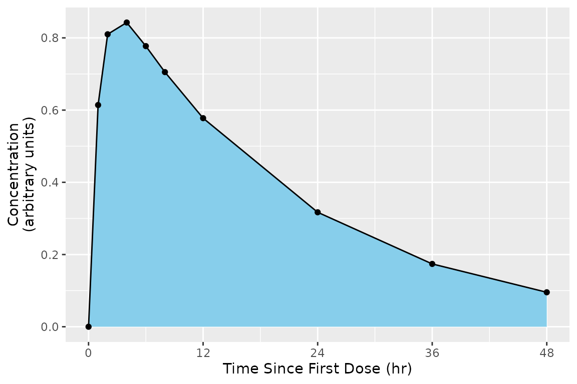
intervals_manual <-
  data.frame(
    start=0,
    end=Inf,
    auclast=TRUE,
    aucinf.obs=TRUE
  )
print(intervals_manual)
## start end auclast aucinf.obs
## 1 0 Inf TRUE TRUE
my.data <- PKNCAdata(d_conc, intervals=intervals_manual)Multiple Intervals
More than one interval may be specified for the same subject or group of subjects by providing more than one row of interval specifications. In the figure below, the blue and green shaded regions indicate the first and second rows of the intervals, respectively.
## Formula for concentration:
##  conc ~ time | treatment + ID
## Data are dense PK.
## With 1 subjects defined in the 'ID' column.
## Nominal time column is not specified.
##
## First 6 rows of concentration data:
##    study treatment ID time      conc   analyte exclude
##  Study 1     Trt 1  1    0 0.0000000 Analyte 1    <NA>
##  Study 1     Trt 1  1    1 0.6140526 Analyte 1    <NA>
##  Study 1     Trt 1  1    2 0.8100022 Analyte 1    <NA>
##  Study 1     Trt 1  1    4 0.8425422 Analyte 1    <NA>
##  Study 1     Trt 1  1    6 0.7771994 Analyte 1    <NA>
##  Study 1     Trt 1  1    8 0.7052469 Analyte 1    <NA>
# Plot the concentration-time data and the interval
ggplot(d_conc_multi, aes(x=time, y=conc)) +
  geom_ribbon(data=d_conc_multi[d_conc_multi$time <= 24,],
              aes(ymax=conc, ymin=0),
              fill="skyblue") +
  geom_ribbon(data=d_conc_multi[d_conc_multi$time >= 144,],
              aes(ymax=conc, ymin=0),
              fill="lightgreen") +
  geom_point() + geom_line() +
  scale_x_continuous(breaks=seq(0, 168, by=12)) +
  scale_y_continuous(limits=c(0, NA)) +
  labs(x="Time Since First Dose (hr)",
       y="Concentration\n(arbitrary units)")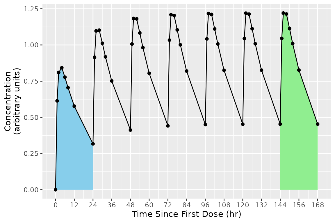
intervals_manual <-
  data.frame(
    start=c(0, 144),
    end=c(24, 168),
    auclast=TRUE
  )
knitr::kable(intervals_manual)| start | end | auclast |
|---|---|---|
| 0 | 24 | TRUE |
| 144 | 168 | TRUE |
Overlapping Intervals and Different Calculations by Interval
In some scenarios, multiple intervals may be needed where some intervals overlap. There is no issue with an interval specification that has two rows with overlapping times; the rows are considered separately. In the example below, the 0-24 interval is shared between both the first and second (shaded blue-green).
The example of overlapping intervals also illustrates that different
calculations can be performed in different intervals. In this case,
auclast is calculated in both intervals while
aucinf.obs is only calculated in the 0-Inf interval.
## Formula for concentration:
##  conc ~ time | treatment + ID
## Data are dense PK.
## With 1 subjects defined in the 'ID' column.
## Nominal time column is not specified.
##
## First 6 rows of concentration data:
##    study treatment ID time      conc   analyte exclude
##  Study 1     Trt 1  1    0 0.0000000 Analyte 1    <NA>
##  Study 1     Trt 1  1    1 0.6140526 Analyte 1    <NA>
##  Study 1     Trt 1  1    2 0.8100022 Analyte 1    <NA>
##  Study 1     Trt 1  1    4 0.8425422 Analyte 1    <NA>
##  Study 1     Trt 1  1    6 0.7771994 Analyte 1    <NA>
##  Study 1     Trt 1  1    8 0.7052469 Analyte 1    <NA>
# Use superposition to simulate multiple doses
ggplot(as.data.frame(d_conc), aes(x=time, y=conc)) +
  geom_ribbon(data=as.data.frame(d_conc),
              aes(ymax=conc, ymin=0),
              fill="lightgreen",
              alpha=0.5) +
  geom_ribbon(data=as.data.frame(d_conc)[as.data.frame(d_conc)$time <= 24,],
              aes(ymax=conc, ymin=0),
              fill="skyblue",
              alpha=0.5) +
  geom_point() + geom_line() +
  scale_x_continuous(breaks=seq(0, 168, by=12)) +
  scale_y_continuous(limits=c(0, NA)) +
  labs(x="Time Since First Dose (hr)",
       y="Concentration\n(arbitrary units)")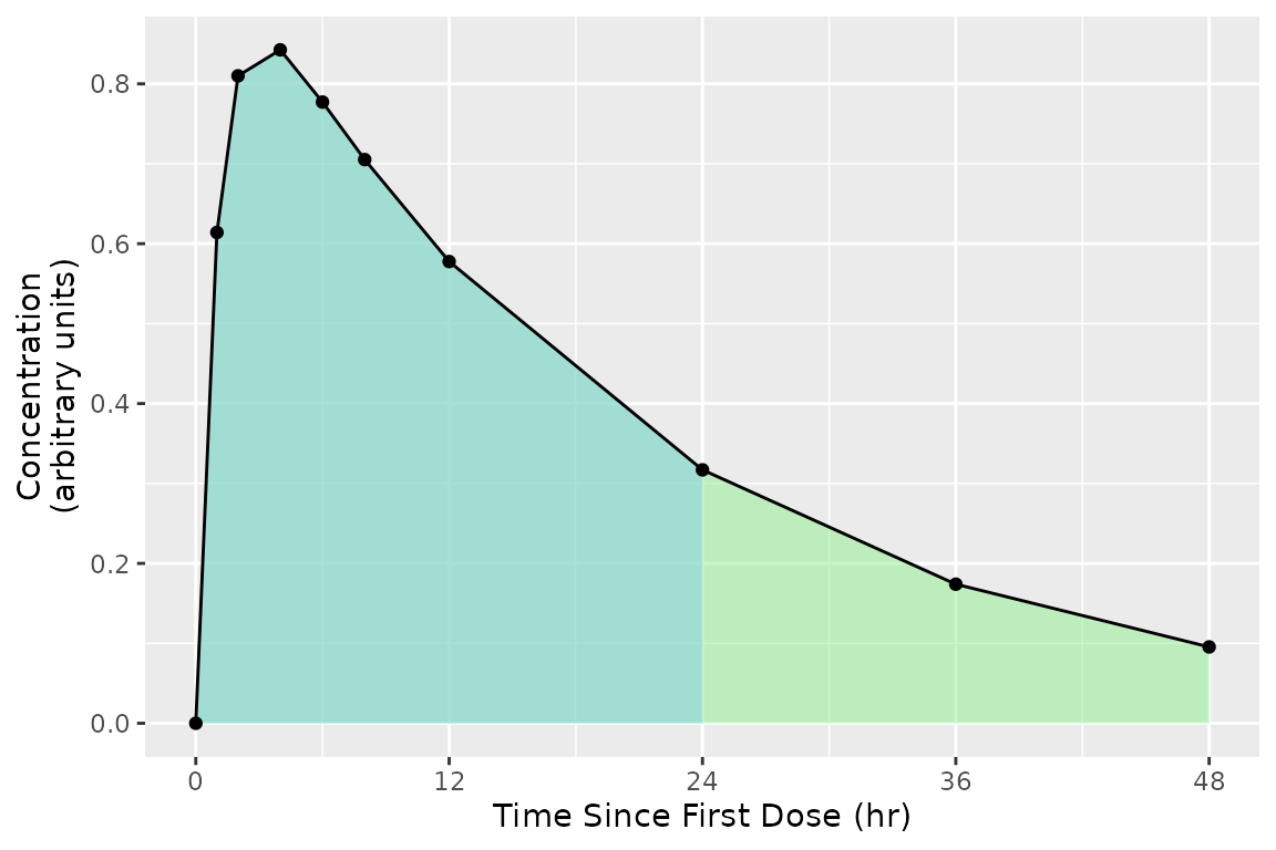
intervals_manual <-
  data.frame(
    start=0,
    end=c(24, Inf),
    auclast=TRUE,
    aucinf.obs=c(FALSE, TRUE)
  )
knitr::kable(intervals_manual)| start | end | auclast | aucinf.obs |
|---|---|---|---|
| 0 | 24 | TRUE | FALSE |
| 0 | Inf | TRUE | TRUE |
my.data <- PKNCAdata(d_conc, intervals=intervals_manual)Intervals with Duration
Some events have durations of times rather than instants in time
associated with them. Two typical examples of duration data in NCA are
intravenous infusions and urine or fecal sample collections. Inform
PKNCA of durations with the duration argument to the
PKNCAdose and PKNCAconc functions.
Duration data are selected for an interval by the event time, which
is the time of the start of the duration (for example, the start of a
urine collection). Like any other data point, a duration record is
selected when its start time is at or after the interval
start and at or before the interval end; the
end of the duration is not considered. A collection that starts within
the interval and ends after the interval end is therefore
selected, and it contributes its full amount to calculations within the
interval (the amount is not pro-rated to the portion of the duration
inside the interval). For the simplest interpretation of results, align
collection start and end times with the interval boundaries.
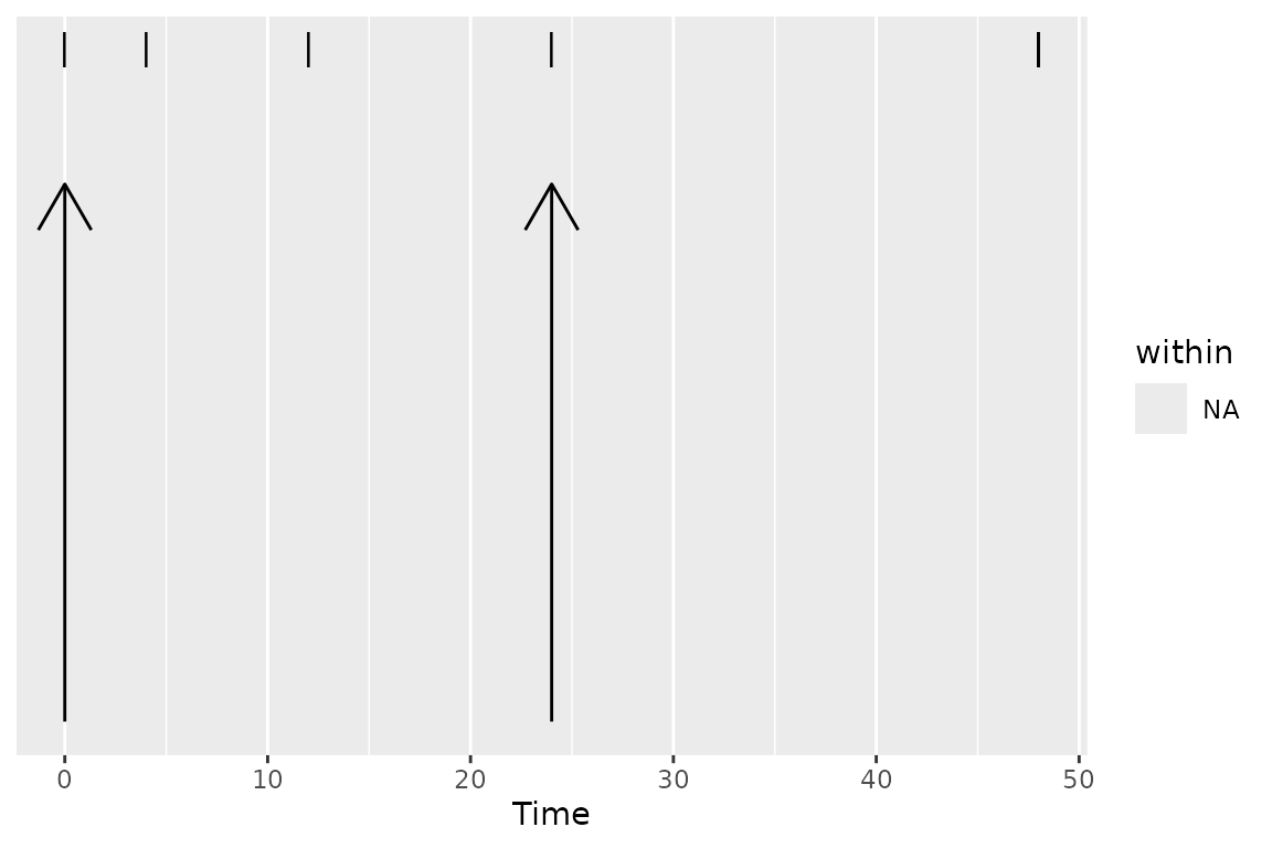
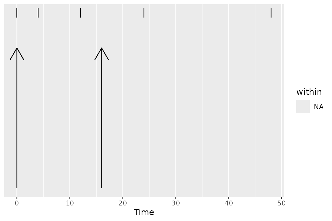
The figures below show which durations are selected for two
intervals. The vertical arrows indicate the interval start
and end, and each horizontal segment is a duration (for
example, a urine collection) with tick marks at the collection
boundaries. In the first figure, the interval is from 0 to 24, and all
four durations are selected, including the duration from 24 to 48
because its start time is exactly at the interval end. In
the second figure, the interval is from 0 to 16: the duration from 12 to
24 is selected because its start time is within the interval, even
though the collection extends past the interval end (and
its full amount contributes to the interval), while the duration from 24
to 48 is not selected.
Multiple-Dose MRT and Vss
The multiple-dose parameters mrt.md.obs,
mrt.md.pred, vss.md.obs, and
vss.md.pred measure MRT and Vss over a steady-state dosing
interval instead of over a single dose.
These are the parameters to use when PK are
nonlinear. When PK are linear, MRT and Vss can be measured from
a single dose, and the single-dose parameters (mrt.obs,
vss.obs, and similar) describe steady state as well. When
PK are nonlinear they do not: clearance and volume at steady state
differ from their values after the first dose, so MRT and Vss have to be
measured over a steady-state interval.
Taking mrt.last over a dosing interval is not a
substitute. AUMC divided by AUC over 0 to tau
leaves out the drug still in the body at the end of the interval and
underestimates MRT substantially. The multiple-dose parameters add the
tau*(AUCinf - AUCtau)/AUCtau term that accounts for it.
The dosing interval comes from a tau column in the
interval specification, and that column takes precedence whenever it is
given:
intervals_md <-
  data.frame(
    start=0, end=24,
    tau=24,
    mrt.md.obs=TRUE, vss.md.obs=TRUE
  )
When no tau column is given, tau is
detected from the dose times with find.tau(), which needs
at least two doses in the dosing data. A steady-state design that
records only the profiled dose has nothing that repeats, so it needs the
tau column. If tau can be neither given nor
detected, the parameters are NA with a warning rather than
silently falling back to the single-dose equation.
Intravenous Infusions
For an IV infusion, use mrt.ivmd.obs,
mrt.ivmd.pred, vss.ivmd.obs, and
vss.ivmd.pred instead. They subtract half of the infusion
duration, the same correction that mrt.iv.obs applies to
the single-dose MRT. Without it, MRT is high by half the infusion
duration and Vss is high by clearance times half the infusion
duration.
Parameters Available for Calculation in an Interval
The following parameters are available in an interval. For more information about the parameter, see the documentation for the function.
| Parameter Name | Formula | Formula Note | Unit Type | Parameter Description | Function for Calculation |
|---|---|---|---|---|---|
| adj_tobit_residual | unitless | Adjusted Tobit residual SD | See the parameter name: half.life | ||
| adj.r.squared | unitless | Adjusted R-sq of half-life fit | See the parameter name: half.life | ||
| ae | amount | Amount excreted (urine/feces) | pk.calc.ae | ||
| aucabove.predose.all | auc | AUC above predose, floor at 0 | pk.calc.aucabove | ||
| aucabove.trough.all | auc | AUC above trough, floor at 0 | pk.calc.aucabove | ||
| aucall | Trapezoidal rule (linear-up/log-down by default) | auc | AUClast plus triangle, 0 at BLQ | pk.calc.auc.all | |
| aucall_df | Satterthwaite approximation for any sampling design (Nedelman and Jia 1998, eq. 6) | count | DF for AUCall (sparse PK only) | See the parameter name: aucall | |
| aucall_se | Variance from weighted covariance across subjects (Nedelman and Jia 1998, Holder 2001), with the trapezoidal weights to the time after tlast | auc | SE of AUCall (sparse PK only) | See the parameter name: aucall | |
| aucall.dn | auc_dosenorm | Dose-normalized aucall | pk.calc.dn | ||
| aucinf.obs | auc | AUC start to inf, obs Clast extrap | pk.calc.auc.inf.obs | ||
| aucinf.obs_df | Satterthwaite approximation for any sampling design (Nedelman and Jia 1998, eq. 6) | count | DF for AUCinf,obs (sparse PK only) | See the parameter name: aucinf.obs | |
| aucinf.obs_se | Weights g are the trapezoidal weights plus the extrapolation weight at tlast (Yuan 1993), with the delta-method gradient for lambda.z when the sparse_lambda_z_se option is “delta” | auc | SE of AUCinf,obs (sparse PK only) | See the parameter name: aucinf.obs | |
| aucinf.obs.dn | auc_dosenorm | Dose-normalized aucinf.obs | pk.calc.dn | ||
| aucinf.pred | auc | AUC start to inf, pred Clast extrap | pk.calc.auc.inf.pred | ||
| aucinf.pred.dn | auc_dosenorm | Dose-normalized aucinf.pred | pk.calc.dn | ||
| aucint.all | Trapezoidal rule with interpolation at interval boundaries | auc | AUC from T1 to T2 (AUCall extrap) | pk.calc.aucint.all | |
| aucint.inf.obs | Trapezoidal rule with interpolation at interval boundaries | auc | AUC from T1 to T2 (AUCinf,obs extrap) | pk.calc.aucint.inf.obs | |
| aucint.inf.pred | Trapezoidal rule with interpolation at interval boundaries | auc | AUC from T1 to T2 (AUCinf,pred extrap) | pk.calc.aucint.inf.pred | |
| aucint.last | Trapezoidal rule with interpolation at interval boundaries | auc | AUC from T1 to T2 (zero extrap) | pk.calc.aucint.last | |
| aucivall | auc | AUCall, IV back-extrap C0 | pk.calc.auciv | ||
| aucivall_df | Satterthwaite approximation for any sampling design (Nedelman and Jia 1998, eq. 6) | count | DF for AUCall IV (sparse PK only) | See the parameter name: aucivall | |
| aucivall_se | With sparse PK, the trapezoidal weights plus the delta-method gradient of the back-extrapolated C0 | auc | SE of AUCall IV (sparse PK only) | See the parameter name: aucivall | |
| aucivinf.obs | auc | AUCinf,obs, IV back-extrap C0 | pk.calc.auciv | ||
| aucivinf.obs_df | Satterthwaite approximation for any sampling design (Nedelman and Jia 1998, eq. 6) | count | DF for AUCinf,obs IV (sparse PK only) | See the parameter name: aucivinf.obs | |
| aucivinf.obs_se | With sparse PK, the trapezoidal weights plus the delta-method gradient of the back-extrapolated C0, the extrapolation weight at tlast, and the delta-method gradient for lambda.z when the sparse_lambda_z_se option is “delta” | auc | SE of AUCinf,obs IV (sparse PK only) | See the parameter name: aucivinf.obs | |
| aucivinf.pred | auc | AUCinf,pred, IV back-extrap C0 | pk.calc.auciv | ||
| aucivint.all | auc | AUCint,all, IV back-extrap C0 | pk.calc.auciv | ||
| aucivint.last | auc | AUCint,last, IV back-extrap C0 | pk.calc.auciv | ||
| aucivlast | auc | AUClast, IV back-extrap C0 | pk.calc.auciv | ||
| aucivlast_df | Satterthwaite approximation for any sampling design (Nedelman and Jia 1998, eq. 6) | count | DF for AUClast IV (sparse PK only) | See the parameter name: aucivlast | |
| aucivlast_se | With sparse PK, the trapezoidal weights plus the delta-method gradient of the back-extrapolated C0 | auc | SE of AUClast IV (sparse PK only) | See the parameter name: aucivlast | |
| aucivpbextall | % | Back-extrap %, IV, AUCall | pk.calc.auciv_pbext | ||
| aucivpbextinf.obs | % | Back-extrap %, IV, AUCinf,obs | pk.calc.auciv_pbext | ||
| aucivpbextinf.pred | % | Back-extrap %, IV, AUCinf,pred | pk.calc.auciv_pbext | ||
| aucivpbextint.all | % | Back-extrap %, IV, AUCint,all | pk.calc.auciv_pbext | ||
| aucivpbextint.last | % | Back-extrap %, IV, AUCint,last | pk.calc.auciv_pbext | ||
| aucivpbextlast | % | Back-extrap %, IV, AUClast | pk.calc.auciv_pbext | ||
| auclast | Trapezoidal rule (linear-up/log-down by default) | auc | AUC start to last conc above LOQ | pk.calc.auc.last | |
| auclast_df | Satterthwaite approximation for any sampling design (Nedelman and Jia 1998, eq. 6) | count | DF for AUClast (sparse PK only) | See the parameter name: auclast | |
| auclast_se | Variance from weighted covariance across subjects (Nedelman and Jia 1998, Holder 2001) | auc | SE of AUClast (sparse PK only) | See the parameter name: auclast | |
| auclast.dn | auc_dosenorm | Dose-normalized auclast | pk.calc.dn | ||
| aucpext.obs | % | % AUCinf extrap after Tlast, obs | pk.calc.aucpext | ||
| aucpext.pred | % | % AUCinf extrap after Tlast, pred | pk.calc.aucpext | ||
| aumcall | Trapezoidal rule (linear-up/log-down by default) | aumc | AUMClast plus triangle moment, 0 at BLQ | pk.calc.aumc.all | |
| aumcall_df | Satterthwaite approximation for any sampling design (Nedelman and Jia 1998, eq. 6) | count | DF for AUMCall (sparse PK only) | See the parameter name: aumcall | |
| aumcall_se | Variance from weighted covariance across subjects (Nedelman and Jia 1998, Holder 2001), with the trapezoidal weights to the time after tlast | aumc | SE of AUMCall (sparse PK only) | See the parameter name: aumcall | |
| aumcall.dn | aumc_dosenorm | Dose-normalized aumcall | pk.calc.dn | ||
| aumcinf.obs | aumc | AUMC start to inf, obs Clast extrap | pk.calc.aumc.inf.obs | ||
| aumcinf.obs_df | Satterthwaite approximation for any sampling design (Nedelman and Jia 1998, eq. 6) | count | DF for AUMCinf,obs (sparse PK only) | See the parameter name: aumcinf.obs | |
| aumcinf.obs_se | Weights g on the moment means are the trapezoidal weights plus the extrapolation weight at tlast, with the delta-method gradient for lambda.z when the sparse_lambda_z_se option is “delta” | aumc | SE of AUMCinf,obs (sparse PK only) | See the parameter name: aumcinf.obs | |
| aumcinf.obs.dn | aumc_dosenorm | Dose-normalized aumcinf.obs | pk.calc.dn | ||
| aumcinf.pred | aumc | AUMC start to inf, pred Clast extrap | pk.calc.aumc.inf.pred | ||
| aumcinf.pred.dn | aumc_dosenorm | Dose-normalized aumcinf.pred | pk.calc.dn | ||
| aumcint.all | Trapezoidal rule with interpolation at interval boundaries | aumc | AUMC from T1 to T2 (AUMCall extrap) | pk.calc.aumcint.all | |
| aumcint.inf.obs | Trapezoidal rule with interpolation at interval boundaries | aumc | AUMC from T1 to T2 (AUMCinf,obs extrap) | pk.calc.aumcint.inf.obs | |
| aumcint.inf.pred | Trapezoidal rule with interpolation at interval boundaries | aumc | AUMC from T1 to T2 (AUMCinf,pred extrap) | pk.calc.aumcint.inf.pred | |
| aumcint.last | Trapezoidal rule with interpolation at interval boundaries | aumc | AUMC from T1 to T2 (zero extrap) | pk.calc.aumcint.last | |
| aumcivall | aumc | AUMCall, IV back-extrap C0 | pk.calc.aumciv | ||
| aumcivall_df | Satterthwaite approximation for any sampling design (Nedelman and Jia 1998, eq. 6) | count | DF for AUMCall IV (sparse PK only) | See the parameter name: aumcivall | |
| aumcivall_se | With sparse PK, the trapezoidal weights on the moment means (C0 does not change the AUMC with the linear trapezoidal rule) | aumc | SE of AUMCall IV (sparse PK only) | See the parameter name: aumcivall | |
| aumcivinf.obs | aumc | AUMCinf,obs, IV back-extrap C0 | pk.calc.aumciv | ||
| aumcivinf.obs_df | Satterthwaite approximation for any sampling design (Nedelman and Jia 1998, eq. 6) | count | DF for AUMCinf,obs IV (sparse PK only) | See the parameter name: aumcivinf.obs | |
| aumcivinf.obs_se | With sparse PK, the trapezoidal weights on the moment means (C0 does not change the AUMC with the linear trapezoidal rule), plus the extrapolation weight at tlast and the delta-method gradient for lambda.z when the sparse_lambda_z_se option is “delta” | aumc | SE of AUMCinf,obs IV (sparse PK only) | See the parameter name: aumcivinf.obs | |
| aumcivinf.pred | aumc | AUMCinf,pred, IV back-extrap C0 | pk.calc.aumciv | ||
| aumcivint.all | aumc | AUMCint,all, IV back-extrap C0 | pk.calc.aumciv | ||
| aumcivint.last | aumc | AUMCint,last, IV back-extrap C0 | pk.calc.aumciv | ||
| aumcivlast | aumc | AUMClast, IV back-extrap C0 | pk.calc.aumciv | ||
| aumcivlast_df | Satterthwaite approximation for any sampling design (Nedelman and Jia 1998, eq. 6) | count | DF for AUMClast IV (sparse PK only) | See the parameter name: aumcivlast | |
| aumcivlast_se | With sparse PK, the trapezoidal weights on the moment means (C0 does not change the AUMC with the linear trapezoidal rule) | aumc | SE of AUMClast IV (sparse PK only) | See the parameter name: aumcivlast | |
| aumclast | Trapezoidal rule (linear-up/log-down by default) | aumc | AUMC start to last conc above LOQ | pk.calc.aumc.last | |
| aumclast_df | Satterthwaite approximation for any sampling design (Nedelman and Jia 1998, eq. 6) | count | DF for AUMClast (sparse PK only) | See the parameter name: aumclast | |
| aumclast_se | Variance from the weighted covariance of the moment curve across subjects | aumc | SE of AUMClast (sparse PK only) | See the parameter name: aumclast | |
| aumclast.dn | aumc_dosenorm | Dose-normalized aumclast | pk.calc.dn | ||
| c0 | Methods are tried in order: c0, logslope, c1, cmin, set0; the formula shows c0 and logslope | conc | Initial conc after IV bolus | pk.calc.c0 | |
| cav | conc | Avg conc in interval (AUClast) | pk.calc.cav | ||
| cav.dn | conc_dosenorm | Dose-normalized cav | pk.calc.dn | ||
| cav.int.all | conc | Avg conc in interval (AUCint,all) | pk.calc.cav | ||
| cav.int.inf.obs | conc | Avg conc in interval (AUCint,inf,obs) | pk.calc.cav | ||
| cav.int.inf.pred | conc | Avg conc in interval (AUCint,inf,pred) | pk.calc.cav | ||
| cav.int.last | conc | Avg conc in interval (AUCint,last) | pk.calc.cav | ||
| ceoi | conc | Concentration at the end of infusion | pk.calc.ceoi | ||
| cl.all | clearance | Clearance, AUCall | pk.calc.cl | ||
| cl.int.all | clearance | Clearance, AUCint,all | pk.calc.cl | ||
| cl.int.inf.obs | clearance | Clearance, AUCint,inf,obs | pk.calc.cl | ||
| cl.int.inf.pred | clearance | Clearance, AUCint,inf,pred | pk.calc.cl | ||
| cl.int.last | clearance | Clearance, AUCint,last | pk.calc.cl | ||
| cl.iv.all | clearance | IV clearance, AUCall | pk.calc.cl | ||
| cl.iv.last | clearance | IV clearance, AUClast | pk.calc.cl | ||
| cl.iv.obs | clearance | IV clearance, AUCinf,obs | pk.calc.cl | ||
| cl.iv.pred | clearance | IV clearance, AUCinf,pred | pk.calc.cl | ||
| cl.ivint.all | clearance | IV clearance, AUCint,all | pk.calc.cl | ||
| cl.ivint.last | clearance | IV clearance, AUCint,last | pk.calc.cl | ||
| cl.last | clearance | Clearance, AUClast | pk.calc.cl | ||
| cl.obs | clearance | Clearance, observed Clast | pk.calc.cl | ||
| cl.pred | clearance | Clearance, predicted Clast | pk.calc.cl | ||
| cl.sparse.last | clearance | Clearance, sparse AUClast | pk.calc.cl | ||
| clast.obs | conc | Last conc observed above LOQ | pk.calc.clast.obs | ||
| clast.obs.dn | conc_dosenorm | Dose-normalized clast.obs | pk.calc.dn | ||
| clast.pred | conc | Predicted Clast from half-life | See the parameter name: half.life | ||
| clast.pred.dn | conc_dosenorm | Dose-normalized clast.pred | pk.calc.dn | ||
| clr.last | renal_clearance | Renal clearance, AUClast | pk.calc.clr | ||
| clr.last.dn | renal_clearance_dosenorm | Dose-normalized clr.last | pk.calc.dn | ||
| clr.obs | renal_clearance | Renal clearance, AUCinf,obs | pk.calc.clr | ||
| clr.obs.dn | renal_clearance_dosenorm | Dose-normalized clr.obs | pk.calc.dn | ||
| clr.pred | renal_clearance | Renal clearance, AUCinf,pred | pk.calc.clr | ||
| clr.pred.dn | renal_clearance_dosenorm | Dose-normalized clr.pred | pk.calc.dn | ||
| cmax | conc | Maximum observed concentration | pk.calc.cmax | ||
| cmax.dn | conc_dosenorm | Dose-normalized cmax | pk.calc.dn | ||
| cmin | conc | Minimum observed concentration | pk.calc.cmin | ||
| cmin.dn | conc_dosenorm | Dose-normalized cmin | pk.calc.dn | ||
| count_conc | count | Count of non-missing conc | pk.calc.count_conc | ||
| count_conc_measured | count | Count of measured, non-BLQ conc | pk.calc.count_conc_measured | ||
| cstart | conc | The predose concentration | pk.calc.cstart | ||
| ctrough | conc | Trough (end of interval) conc | pk.calc.ctrough | ||
| ctrough.dn | conc_dosenorm | Dose-normalized ctrough | pk.calc.dn | ||
| deg.fluc | % | Degree of fluctuation | pk.calc.deg.fluc | ||
| erint | Amount recovered during the interval divided by the interval duration | amount_time | Excretion rate from T1 to T2 | pk.calc.erint | |
| erlst | The last collection with a nonzero excretion rate, ordered by collection midpoint | amount_time | Last measurable excretion rate | pk.calc.erlst | |
| ermax | amount_time | Maximum excretion rate | pk.calc.ermax | ||
| ertlst | time | Midpoint time of last excr rate | pk.calc.ertlst | ||
| ertmax | time | Midpoint time of max excr rate | pk.calc.ertmax | ||
| f.int.all | fraction | Bioavailability from AUCint,all | pk.calc.f | ||
| f.int.last | fraction | Bioavailability from AUCint,last | pk.calc.f | ||
| f.int.obs | fraction | Bioavailability from AUCint,inf,obs | pk.calc.f | ||
| f.int.pred | fraction | Bioavailability from AUCint,inf,pred | pk.calc.f | ||
| f.last | fraction | Bioavailability from AUClast | pk.calc.f | ||
| f.obs | fraction | Bioavailability from AUCinf,obs | pk.calc.f | ||
| f.pred | fraction | Bioavailability from AUCinf,pred | pk.calc.f | ||
| fe | amount_dose | Fraction of dose excreted | pk.calc.fe | ||
| half.life | time | The (terminal) half-life | pk.calc.half.life | ||
| kel.all | inverse_time | Elim rate, MRTall | pk.calc.kel | ||
| kel.int.all | inverse_time | Elim rate, MRTint,all | pk.calc.kel | ||
| kel.int.inf.obs | inverse_time | Elim rate, MRTint,inf,obs | pk.calc.kel | ||
| kel.int.inf.pred | inverse_time | Elim rate, MRTint,inf,pred | pk.calc.kel | ||
| kel.int.last | inverse_time | Elim rate, MRTint,last | pk.calc.kel | ||
| kel.iv.all | inverse_time | Elim rate, IV MRTall | pk.calc.kel | ||
| kel.iv.last | inverse_time | Elim rate, IV MRTlast | pk.calc.kel | ||
| kel.iv.obs | inverse_time | Elim rate, IV MRTobs | pk.calc.kel | ||
| kel.iv.pred | inverse_time | Elim rate, IV MRTpred | pk.calc.kel | ||
| kel.ivint.all | inverse_time | Elim rate, IV MRTint,all | pk.calc.kel | ||
| kel.ivint.last | inverse_time | Elim rate, IV MRTint,last | pk.calc.kel | ||
| kel.last | inverse_time | Elim rate, MRT via AUClast | pk.calc.kel | ||
| kel.obs | inverse_time | Elim rate, MRT w/ obs Clast | pk.calc.kel | ||
| kel.pred | inverse_time | Elim rate, MRT w/ pred Clast | pk.calc.kel | ||
| kel.sparse.last | inverse_time | Elim rate, sparse MRTlast | pk.calc.kel | ||
| lambda.z | inverse_time | Terminal elim rate (lambda.z) | See the parameter name: half.life | ||
| lambda.z.corrxy | unitless | Corr(time,log-conc) for lambda.z | See the parameter name: half.life | ||
| lambda.z.n.points | $n_{\lambda_z} = \left| t_{\lambda_z} \right|$ | count | Number of points used, lambda.z | See the parameter name: half.life | |
| lambda.z.n.points_blq | count | BLQ points in Tobit lambda.z | See the parameter name: half.life | ||
| lambda.z.time.first | time | First time point for lambda.z | See the parameter name: half.life | ||
| lambda.z.time.last | time | Last time point for lambda.z | See the parameter name: half.life | ||
| mrt.all | time | MRT, AUCall/AUMCall | pk.calc.mrt | ||
| mrt.int.all | time | MRT, interval AUCall/AUMCall | pk.calc.mrt | ||
| mrt.int.inf.obs | time | MRT, interval AUCinf,obs/AUMCinf,obs | pk.calc.mrt | ||
| mrt.int.inf.pred | time | MRT, interval AUCinf,pred/AUMCinf,pred | pk.calc.mrt | ||
| mrt.int.last | time | MRT, interval AUClast/AUMClast | pk.calc.mrt | ||
| mrt.iv.all | time | IV MRT, AUCall/AUMCall | pk.calc.mrt.iv | ||
| mrt.iv.last | time | IV MRT, AUClast/AUMClast | pk.calc.mrt.iv | ||
| mrt.iv.obs | time | IV MRT, AUCinf,obs/AUMCinf,obs | pk.calc.mrt.iv | ||
| mrt.iv.pred | time | IV MRT, AUCinf,pred/AUMCinf,pred | pk.calc.mrt.iv | ||
| mrt.ivint.all | time | IV MRT, interval AUCall/AUMCall | pk.calc.mrt.iv | ||
| mrt.ivint.last | time | IV MRT, interval AUClast/AUMClast | pk.calc.mrt.iv | ||
| mrt.ivmd.obs | time | IV MRT, multi-dose, AUCinf,obs | pk.calc.mrt.md.iv | ||
| mrt.ivmd.pred | time | IV MRT, multi-dose, AUCinf,pred | pk.calc.mrt.md.iv | ||
| mrt.last | time | MRT, AUClast/AUMClast | pk.calc.mrt | ||
| mrt.md.obs | time | MRT, multi-dose AUCinf,obs/AUMCinf,obs | pk.calc.mrt.md | ||
| mrt.md.pred | time | MRT, multi-dose AUCinf,pred/AUMCinf,pred | pk.calc.mrt.md | ||
| mrt.obs | time | MRT to inf, observed Clast | pk.calc.mrt | ||
| mrt.pred | time | MRT to inf, predicted Clast | pk.calc.mrt | ||
| mrt.sparse.last | time | MRT, sparse AUClast/AUMClast | pk.calc.mrt | ||
| ptr | fraction | Peak-to-trough ratio | pk.calc.ptr | ||
| r.squared | Regression of on time over the terminal points | unitless | R-squared of half-life fit | See the parameter name: half.life | |
| ratio.aucinf.obs | fraction | Ratio of AUCinf,obs to reference | pk.calc.ratio | ||
| ratio.aucinf.pred | fraction | Ratio of AUCinf,pred to reference | pk.calc.ratio | ||
| ratio.aucint.all | fraction | Ratio of AUCint,all to reference | pk.calc.ratio | ||
| ratio.aucint.last | fraction | Ratio of AUCint,last to reference | pk.calc.ratio | ||
| ratio.auclast | fraction | Ratio of AUClast to reference | pk.calc.ratio | ||
| ratio.cmax | fraction | Ratio of Cmax to reference | pk.calc.ratio | ||
| span.ratio | fraction | Ratio of lambda.z time span to half-life | See the parameter name: half.life | ||
| sparse_auc_df | Satterthwaite approximation for any sampling design (Nedelman and Jia 1998, eq. 6) | count | DF for sparse AUC to last conc above LOQ | See the parameter name: sparse_auclast | |
| sparse_auc_se | Variance from weighted covariance across subjects (Nedelman and Jia 1998, Holder 2001) | auc | SE of sparse AUC to last conc above LOQ | See the parameter name: sparse_auclast | |
| sparse_auclast | Linear trapezoidal using population mean concentrations | auc | Sparse AUC to last conc above LOQ | pk.calc.sparse_auclast | |
| sparse_aumc_df | count | DF for sparse AUMClast | See the parameter name: sparse_aumclast | ||
| sparse_aumc_se | aumc | SE of sparse AUMC to last conc above LOQ | See the parameter name: sparse_aumclast | ||
| sparse_aumclast | aumc | Sparse AUMC to last conc above LOQ | pk.calc.sparse_aumclast | ||
| swing | % | Swing relative to Cmin | pk.calc.swing | ||
| tfirst | time | Time of first conc above LOQ | pk.calc.tfirst | ||
| thalf.eff.iv.last | time | Effective half-life, IV MRTlast | pk.calc.thalf.eff | ||
| thalf.eff.iv.obs | time | Effective half-life, IV MRTobs | pk.calc.thalf.eff | ||
| thalf.eff.iv.pred | time | Effective half-life, IV MRTpred | pk.calc.thalf.eff | ||
| thalf.eff.last | time | Effective half-life, MRTlast | pk.calc.thalf.eff | ||
| thalf.eff.obs | time | Effective half-life, MRTobs | pk.calc.thalf.eff | ||
| thalf.eff.pred | time | Effective half-life, MRTpred | pk.calc.thalf.eff | ||
| time_above | Crossing times interpolated using the AUC method (linear or log-linear) | time | Time above a given concentration | pk.calc.time_above | |
| tlag | time | Lag time | pk.calc.tlag | ||
| tlast | time | Time of last conc above LOQ | pk.calc.tlast | ||
| tmax | time | Time of maximum observed conc | pk.calc.tmax | ||
| tmin | time | Time of minimum observed conc | pk.calc.tmin | ||
| tobit_residual | unitless | Tobit fit residual SD, log-conc | See the parameter name: half.life | ||
| totdose | dose | Total dose given in interval | pk.calc.totdose | ||
| volpk | volume | Sum of urine volumes for interval | pk.calc.volpk | ||
| vss.all | volume | Vss, calc from AUCall | pk.calc.vss | ||
| vss.int.all | volume | Vss, calc from interval AUCint,all | pk.calc.vss | ||
| vss.int.inf.obs | volume | Vss, calc from interval AUCint,inf,obs | pk.calc.vss | ||
| vss.int.inf.pred | volume | Vss, calc from interval AUCint,inf,pred | pk.calc.vss | ||
| vss.int.last | volume | Vss, calc from interval AUCint,last | pk.calc.vss | ||
| vss.iv.all | volume | IV Vss, calc from AUCall | pk.calc.vss | ||
| vss.iv.last | volume | IV Vss, calc from AUClast | pk.calc.vss | ||
| vss.iv.obs | volume | IV Vss, observed Clast | pk.calc.vss | ||
| vss.iv.pred | volume | IV Vss, predicted Clast | pk.calc.vss | ||
| vss.ivint.all | volume | IV Vss, calc from interval AUCint,all | pk.calc.vss | ||
| vss.ivint.last | volume | IV Vss, calc from interval AUCint,last | pk.calc.vss | ||
| vss.ivmd.obs | volume | IV Vss, multi-dose, obs | pk.calc.vss | ||
| vss.ivmd.pred | volume | IV Vss, multi-dose, pred | pk.calc.vss | ||
| vss.last | volume | Vss, calc from AUClast | pk.calc.vss | ||
| vss.md.obs | volume | Vss, multi-dose, obs | pk.calc.vss | ||
| vss.md.pred | volume | Vss, multi-dose, pred | pk.calc.vss | ||
| vss.obs | volume | Vss, observed Clast | pk.calc.vss | ||
| vss.pred | volume | Vss, predicted Clast | pk.calc.vss | ||
| vss.sparse.last | volume | Vss, calc from sparse AUClast | pk.calc.vss | ||
| vz.all | volume | Vz, AUCall-based CL | pk.calc.vz | ||
| vz.int.all | volume | Vz, interval AUCint,all | pk.calc.vz | ||
| vz.int.inf.obs | volume | Vz, interval AUCint,inf,obs | pk.calc.vz | ||
| vz.int.inf.pred | volume | Vz, interval AUCint,inf,pred | pk.calc.vz | ||
| vz.int.last | volume | Vz, interval AUCint,last | pk.calc.vz | ||
| vz.iv.all | volume | IV Vz, AUCall | pk.calc.vz | ||
| vz.iv.last | volume | IV Vz, AUClast | pk.calc.vz | ||
| vz.iv.obs | volume | IV Vz, observed AUCinf | pk.calc.vz | ||
| vz.iv.pred | volume | IV Vz, predicted AUCinf | pk.calc.vz | ||
| vz.ivint.all | volume | IV Vz, interval AUCint,all | pk.calc.vz | ||
| vz.ivint.last | volume | IV Vz, interval AUCint,last | pk.calc.vz | ||
| vz.last | volume | Vz, AUClast-based CL | pk.calc.vz | ||
| vz.obs | volume | Vz, observed Clast | pk.calc.vz | ||
| vz.pred | volume | Vz, predicted Clast | pk.calc.vz | ||
| vz.sparse.last | volume | Vz from sparse sampling | pk.calc.vz |