flowchart LR
    A["Single dose\nprofile (0→∞)"] --> B["Shift by τ,\nshift by 2τ, ..."]
    B --> C["Sum contributions\nat each time t"]
    C --> D["Predicted SS\nprofile (0→τ)"]
11 Superposition
11.1 What superposition does
Superposition predicts steady-state concentration-time profiles from a single-dose profile by linearly summing lagged copies of the single-dose curve. This is the NCA equivalent of multi-dose simulation, and it requires no compartmental model.
The core assumption is linear, time-invariant pharmacokinetics: the drug does not accumulate non-linearly, and clearance and volume do not change over time.
11.2 Basic superposition
# Use Theoph subject 1 as single-dose reference
subj1 <- d_conc |> filter(subject == "1")
actual_dose <- d_dose |> filter(subject == "1") |> pull(dose)

o_conc_1 <- PKNCAconc(subj1, conc ~ time | subject)

# Predict steady-state profile with τ = 24 h, show 3 dosing intervals
ss_profile <- superposition(
  o_conc_1,
  tau         = 24,           # dosing interval (h)
  dose.input  = actual_dose,  # dose used to generate the single-dose data
  dose.amount = actual_dose,  # dose to simulate at SS (same here)
  n.tau       = 3,            # simulate 3 intervals
  check.blq   = FALSE         # Theoph has non-zero first sample
)

head(ss_profile, 12)
# A tibble: 12 × 3
subject conc time
<ord> <dbl> <dbl>
1 1 5.12 0
2 1 7.17 0.25
3 1 8.54 0.370
4 1 10.8 0.57
5 1 14.7 1.12
6 1 13.6 2.02
7 1 12.2 3.82
8 1 11.8 5.1
9 1 10.6 7.03
10 1 9.72 9.05
11 1 8.38 12.1
12 1 4.71 24 11.3 Visualising the approach to steady state
With n.tau = Inf, superposition runs until the profile converges to steady state (within steady.state.tol).
ss_converged <- superposition(
  o_conc_1,
  tau         = 24,
  dose.input  = actual_dose,
  dose.amount = actual_dose,
  n.tau       = Inf,
  check.blq   = FALSE
)

ggplot(ss_converged, aes(x = time, y = conc)) +
  geom_line(colour = "steelblue") +
  geom_point(size = 2, colour = "steelblue") +
  labs(title = "Superposition: predicted steady-state profile (τ = 24 h)",
       x = "Time (h)", y = "Predicted SS concentration (mg/L)") +
  theme_minimal()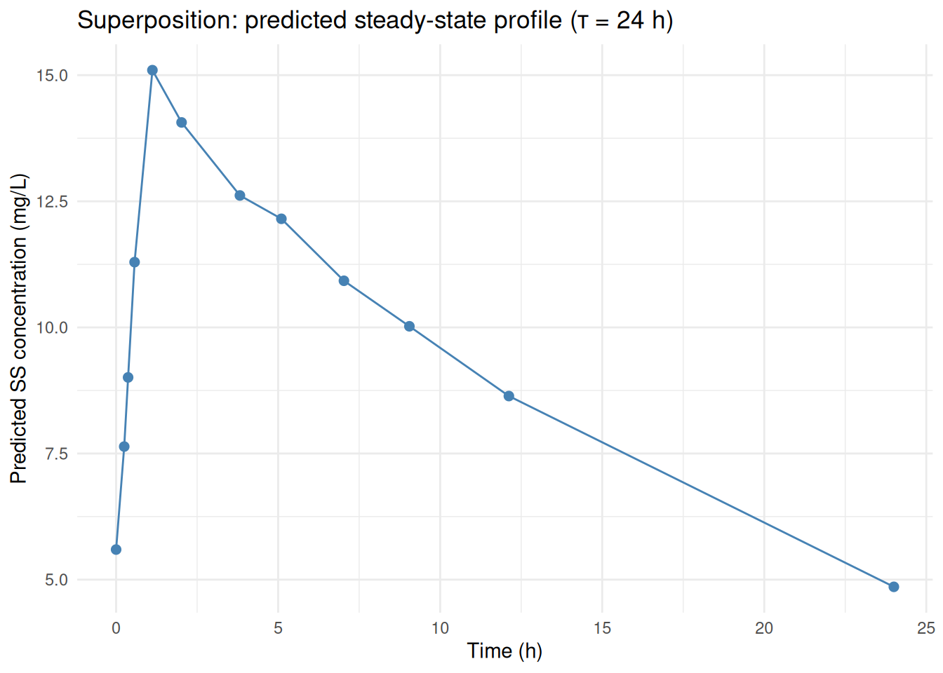
11.4 Changing dose at steady state
To predict the effect of a dose change, set dose.amount to the new dose while keeping dose.input as the original dose. PKNCA scales the concentrations proportionally.
ss_half_dose <- superposition(
  o_conc_1,
  tau         = 24,
  dose.input  = actual_dose,
  dose.amount = actual_dose / 2,   # half dose
  n.tau       = Inf,
  check.blq   = FALSE
)

bind_rows(
  ss_converged   |> mutate(regimen = "Full dose"),
  ss_half_dose   |> mutate(regimen = "Half dose")
) |>
  ggplot(aes(x = time, y = conc, colour = regimen)) +
  geom_line() + geom_point(size = 2) +
  labs(title = "Dose scaling via superposition",
       x = "Time (h)", y = "Predicted SS concentration (mg/L)") +
  scale_colour_manual(values = c("Full dose" = "steelblue", "Half dose" = "coral")) +
  theme_minimal()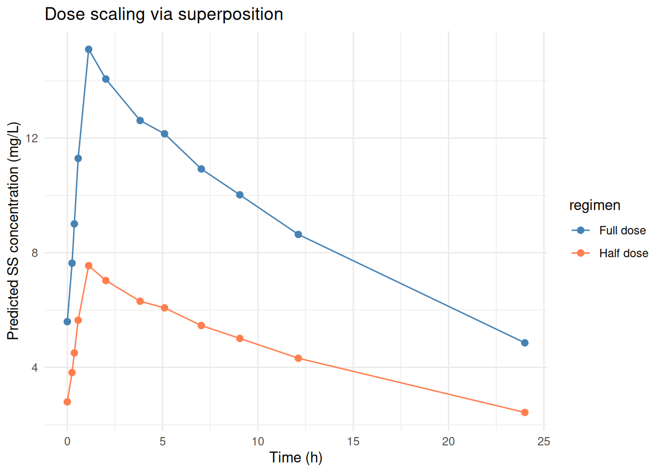
11.5 Changing the dosing interval (τ)
ss_8h <- superposition(
  o_conc_1,
  tau         = 8,
  dose.input  = actual_dose,
  dose.amount = actual_dose,
  n.tau       = Inf,
  check.blq   = FALSE
)

ggplot(ss_8h, aes(x = time, y = conc)) +
  geom_line(colour = "firebrick") +
  geom_point(size = 2, colour = "firebrick") +
  labs(title = "Superposition with τ = 8 h (more frequent dosing)",
       x = "Time within interval (h)", y = "Predicted SS concentration (mg/L)") +
  theme_minimal()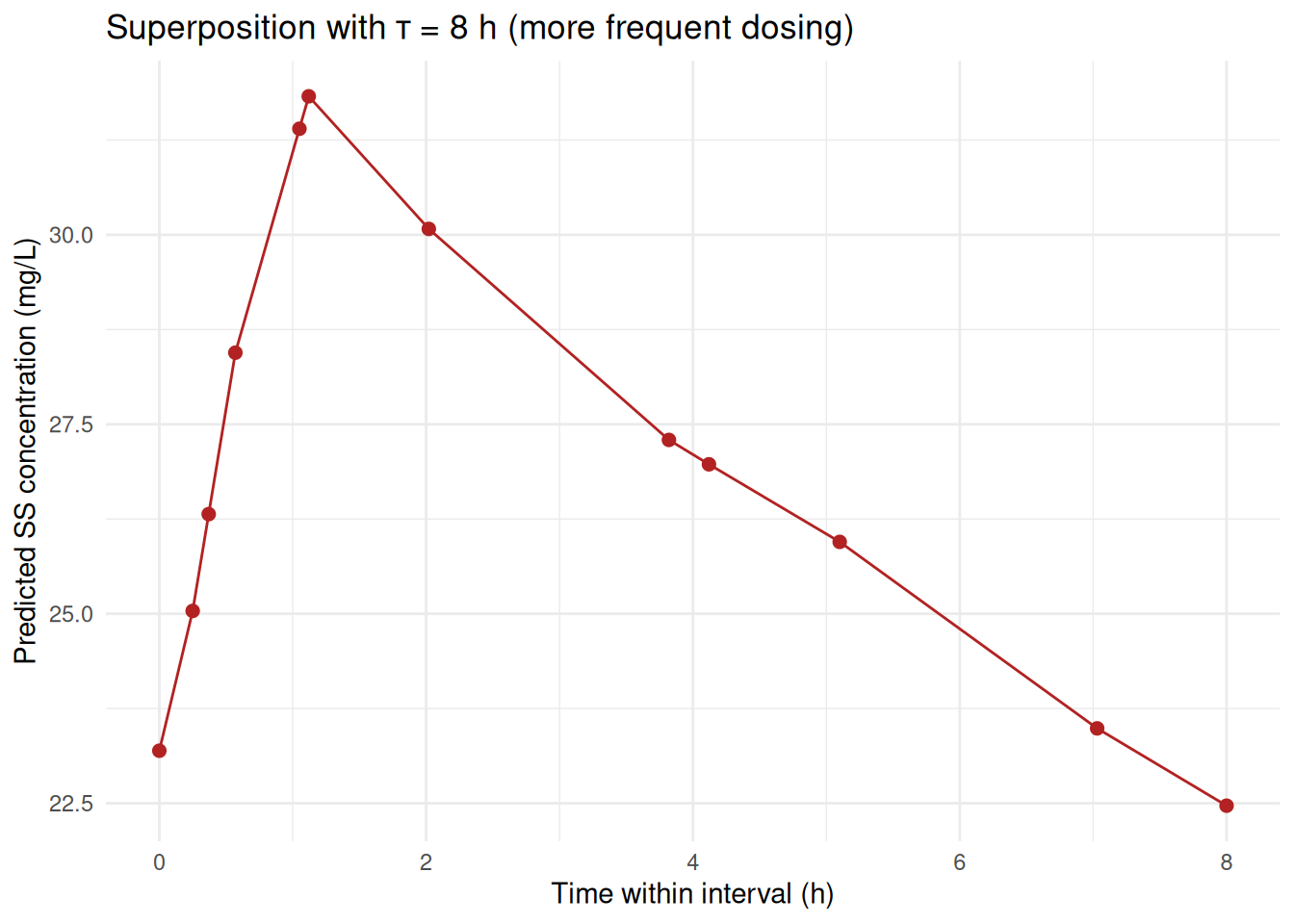
11.6 Extracting accumulation ratio
The accumulation ratio (Rac) is Cmax at steady state divided by Cmax after the first dose:
cmax_sd <- max(subj1$conc, na.rm = TRUE)
cmax_ss <- max(ss_converged$conc, na.rm = TRUE)
rac      <- cmax_ss / cmax_sd
cat("Accumulation ratio (Rac):", round(rac, 2), "\n")
Accumulation ratio (Rac): 1.44 cat("Single-dose Cmax:", round(cmax_sd, 2), "mg/L\n")Single-dose Cmax: 10.5 mg/Lcat("Steady-state Cmax:", round(cmax_ss, 2), "mg/L\n")Steady-state Cmax: 15.1 mg/L11.7 Key arguments reference
| Argument | Required | Meaning |
|---|---|---|
tau |
Yes | Dosing interval (same time units as data) |
dose.input |
When dose.amount ≠ NULL |
Dose used to generate the observed profile |
dose.amount |
When dose.input ≠ NULL |
Dose to simulate (for dose scaling) |
n.tau |
No (default Inf) |
Number of intervals to simulate before stopping |
steady.state.tol |
No (default 0.001) | Convergence tolerance for n.tau = Inf |
check.blq |
No (default TRUE) |
Require first concentration = 0; set FALSE if first sample is non-zero |
auc.type |
No (default "AUCinf") |
How to extrapolate the single-dose tail: "AUCinf" or "AUClast" |
additional.times |
No | Extra timepoints to include in the output |
Limitation: Superposition assumes linear PK. It should not be used for drugs with non-linear kinetics (e.g., Michaelis-Menten elimination, time-varying clearance, or saturable protein binding).