flowchart TD
    A["All points after Tmax"] --> B["Try subsets: last 3, last 4, ..., all"]
    B --> C["Fit log-linear regression to each"]
    C --> D{"Passes quality filters?\nλz > 0, R² ≥ threshold\nspan.ratio ≥ minimum"}
    D -- yes --> E["Compute adj.R²"]
    D -- no --> F["Discard subset"]
    E --> G["Select longest window within adj.r.squared.factor of best adj.R²"]
    G --> H["Return λz, half.life, R², n.points"]
5 Half-Life and Terminal Phase
5.1 How PKNCA estimates λz
PKNCA uses curve stripping: it systematically evaluates all possible subsets of terminal-phase points (from 3 points up to the full tail), fits log-linear regression to each subset, and selects the best fit based on adjusted R².
The selection criterion uses a tolerance window: among all subsets that pass quality filters, PKNCA picks the one with the most points whose adjusted R² is within adj.r.squared.factor of the best adjusted R²:
\[\text{selected} = \arg\max_{\text{n points}} \left\{ \text{adj.}R^2 \geq \max(\text{adj.}R^2) - \text{adj.r.squared.factor} \right\}\]
The small tolerance (adj.r.squared.factor, default 0.0001) means: prefer longer windows (more points → more accurate λz) unless the longer window’s adj.R² is noticeably worse than the best. This is a model-selection tolerance, not a per-point penalty added to R².
5.2 Basic half-life output
hl_interval <- data.frame(
  start             = 0,
  end               = Inf,
  half.life         = TRUE,
  lambda.z          = TRUE,
  lambda.z.n.points = TRUE,
  lambda.z.time.first = TRUE,
  r.squared         = TRUE,
  adj.r.squared     = TRUE,
  span.ratio        = TRUE
)

o_nca <- pk.nca(PKNCAdata(o_conc, o_dose, intervals = hl_interval))

as.data.frame(o_nca) |>
  filter(PPTESTCD %in% c("half.life", "lambda.z", "lambda.z.n.points",
                          "lambda.z.time.first", "adj.r.squared", "span.ratio")) |>
  select(subject, PPTESTCD, PPORRES) |>
  tidyr::pivot_wider(names_from = PPTESTCD, values_from = PPORRES) |>
  arrange(subject)
# A tibble: 12 × 7
subject lambda.z adj.r.squared lambda.z.time.first lambda.z.n.points
<ord> <dbl> <dbl> <dbl> <dbl>
1 6 0.0878 0.998 2.03 7
2 7 0.0883 0.998 6.98 4
3 8 0.0815 0.989 3.53 6
4 11 0.0955 1.000 9.03 3
5 3 0.102 0.999 9 3
6 2 0.104 0.996 7.03 4
7 4 0.0993 0.998 9.02 3
8 9 0.0825 0.999 8.8 3
9 12 0.110 0.999 9.03 3
10 10 0.0750 0.999 9.38 3
11 1 0.0485 1.000 9.05 3
12 5 0.0866 0.998 7.02 4
# ℹ 2 more variables: half.life <dbl>, span.ratio <dbl>What each output means:
| Parameter | Meaning |
|---|---|
lambda.z |
Terminal elimination rate constant (h⁻¹) |
half.life |
ln(2) / λz |
lambda.z.n.points |
Number of points used in the selected regression |
lambda.z.time.first |
First timepoint included in the regression window |
r.squared / adj.r.squared |
Fit quality of the selected regression |
span.ratio |
(lambda.z.time.last − lambda.z.time.first) / half.life — post-hoc quality flag |
5.3 Quality filters
PKNCA applies one filter during fitting and exposes additional parameters you use to flag or exclude results after fitting with exclude().
Important distinction: Only
min.hl.pointsis enforced insidepk.calc.half.life()— too few points returnshalf.life = NAimmediately.min.hl.r.squaredandmin.span.ratioare not consulted during fitting; they are thresholds forexclude()calls afterpk.nca().
5.3.1 1. Minimum number of points (enforced during fitting)
# Default: 3 points minimum — the only filter that makes half.life NA during pk.nca()
o_data_4pts <- PKNCAdata(o_conc, o_dose, intervals = hl_interval,
                          options = list(min.hl.points = 4))
o_nca_4pts  <- pk.nca(o_data_4pts)

as.data.frame(o_nca_4pts) |>
  filter(PPTESTCD %in% c("half.life", "lambda.z.n.points")) |>
  select(subject, PPTESTCD, PPORRES) |>
  tidyr::pivot_wider(names_from = PPTESTCD, values_from = PPORRES) |>
  arrange(subject)
# A tibble: 12 × 3
subject lambda.z.n.points half.life
<ord> <dbl> <dbl>
1 6 7 7.89
2 7 4 7.85
3 8 6 8.51
4 11 4 7.22
5 3 6 7.36
6 2 4 6.66
7 4 4 7.32
8 9 4 8.70
9 12 5 6.67
10 10 4 9.46
11 1 5 14.4
12 5 4 8.005.3.2 2. R² threshold (post-hoc exclusion via exclude())
min.hl.r.squared sets the minimum unadjusted R² threshold. It has no effect during pk.nca(); use it with exclude_nca_min.hl.r.squared() after fitting:
# Compute half-life for all subjects
o_nca_r2 <- pk.nca(PKNCAdata(o_conc, o_dose, intervals = hl_interval))

# Then flag results with unadjusted R² < 0.95
o_nca_r2_excl <- exclude(
  o_nca_r2,
  reason = "r.squared < 0.95",
  FUN    = exclude_nca_min.hl.r.squared(0.95)
)
Loading required namespace: testthatas.data.frame(o_nca_r2_excl) |>
filter(PPTESTCD %in% c("half.life", "r.squared")) |>
select(subject, PPTESTCD, PPORRES) |>
tidyr::pivot_wider(names_from = PPTESTCD, values_from = PPORRES) |>
arrange(subject)# A tibble: 12 × 3
subject r.squared half.life
<ord> <dbl> <dbl>
1 6 0.998 7.89
2 7 0.999 7.85
3 8 0.991 8.51
4 11 1.000 7.26
5 3 0.999 6.77
6 2 0.997 6.66
7 4 0.999 6.98
8 9 0.999 8.41
9 12 0.999 6.29
10 10 1.000 9.25
11 1 1.000 14.3
12 5 0.999 8.00For the stricter adjusted R² filter: exclude_nca_min.hl.adj.r.squared(min).
5.3.3 3. Span ratio threshold (post-hoc exclusion via exclude())
min.span.ratio has no effect during pk.nca(); use it with exclude_nca_span.ratio():
# Flag half-lives with span.ratio < 2
o_nca_span_excl <- exclude(
  o_nca_r2,
  reason = "span.ratio < 2",
  FUN    = exclude_nca_span.ratio(2)
)

as.data.frame(o_nca_span_excl) |>
  filter(PPTESTCD %in% c("half.life", "span.ratio")) |>
  select(subject, PPTESTCD, PPORRES) |>
  tidyr::pivot_wider(names_from = PPTESTCD, values_from = PPORRES) |>
  arrange(subject)
# A tibble: 12 × 3
subject half.life span.ratio
<ord> <dbl> <dbl>
1 6 7.89 2.76
2 7 7.85 2.20
3 8 8.51 2.42
4 11 7.26 2.07
5 3 6.77 2.24
6 2 6.66 2.59
7 4 6.98 2.24
8 9 8.41 1.86
9 12 6.29 2.41
10 10 9.25 1.55
11 1 14.3 1.07
12 5 8.00 2.175.3.4 4. Allow / exclude Tmax
By default Tmax is excluded from the λz regression (drug may still be distributing).
o_data_tmax <- PKNCAdata(o_conc, o_dose, intervals = hl_interval,
                          options = list(allow.tmax.in.half.life = TRUE))
o_nca_tmax  <- pk.nca(o_data_tmax)

as.data.frame(o_nca_tmax) |>
  filter(PPTESTCD %in% c("half.life", "lambda.z.n.points", "lambda.z.time.first")) |>
  select(subject, PPTESTCD, PPORRES) |>
  tidyr::pivot_wider(names_from = PPTESTCD, values_from = PPORRES) |>
  arrange(subject)
# A tibble: 12 × 4
subject lambda.z.time.first lambda.z.n.points half.life
<ord> <dbl> <dbl> <dbl>
1 6 2.03 7 7.89
2 7 6.98 4 7.85
3 8 2.02 7 8.47
4 11 9.03 3 7.26
5 3 9 3 6.77
6 2 7.03 4 6.66
7 4 9.02 3 6.98
8 9 8.8 3 8.41
9 12 9.03 3 6.29
10 10 9.38 3 9.25
11 1 9.05 3 14.3
12 5 7.02 4 8.005.4 Manually controlling which points are used
5.4.1 Excluding specific points (exclude_half.life)
Mark individual observations that should never be included in the λz regression — for example, a suspected outlier or a resurgence peak.
d_conc_excl <- d_conc |>
  mutate(excl_hl = ifelse(subject == "1" & time > 16, TRUE, NA))

o_conc_excl <- PKNCAconc(d_conc_excl, conc ~ time | subject,
                          exclude_half.life = "excl_hl")

o_nca_excl <- pk.nca(PKNCAdata(o_conc_excl, o_dose, intervals = hl_interval))

# Compare n.points and lambda.z.time.first for subject 1
bind_rows(
  as.data.frame(o_nca) |>
    filter(subject == "1", PPTESTCD %in% c("half.life", "lambda.z.n.points")) |>
    mutate(version = "default"),
  as.data.frame(o_nca_excl) |>
    filter(subject == "1", PPTESTCD %in% c("half.life", "lambda.z.n.points")) |>
    mutate(version = "late points excluded")
) |>
  select(version, PPTESTCD, PPORRES) |>
  arrange(version, PPTESTCD)
# A tibble: 4 × 3
version PPTESTCD PPORRES
<chr> <chr> <dbl>
1 default half.life 14.3
2 default lambda.z.n.points 3
3 late points excluded half.life 15.3
4 late points excluded lambda.z.n.points 3 5.4.2 Forcing specific points (include_half.life)
Mark points that must be included — they cannot be dropped even if excluding them would improve the fit. Useful for regulatory requirements.
d_conc_incl <- d_conc |>
  mutate(incl_hl = ifelse(subject == "1" & time %in% c(9.05, 12.12), TRUE, NA))

o_conc_incl <- PKNCAconc(d_conc_incl, conc ~ time | subject,
                          include_half.life = "incl_hl")

o_nca_incl <- pk.nca(PKNCAdata(o_conc_incl, o_dose, intervals = hl_interval))
Warning: n must be > 2 for adj.r.squaredas.data.frame(o_nca_incl) |>
filter(subject == "1",
PPTESTCD %in% c("half.life", "lambda.z.n.points", "lambda.z.time.first")) |>
select(PPTESTCD, PPORRES)# A tibble: 3 × 2
PPTESTCD PPORRES
<chr> <dbl>
1 lambda.z.time.first 9.05
2 lambda.z.n.points 2
3 half.life 14.3 Note:
include_half.lifeforces the curve-stripping algorithm to always start at or before the earliest forced point. If the forced point is early in the profile, this can result in a worse fit (lower R²) — the point is still included even if it pulls the regression down.
5.5 Tobit regression for BLQ-heavy data
Available in PKNCA ≥ 0.12.2 (now on CRAN).
5.5.1 Why Tobit?
In studies where drug concentrations in the terminal elimination phase are frequently below the lower limit of quantification (BLQ), ordinary least-squares (OLS) log-linear regression produces biased estimates of λz. The bias arises because OLS either:
- drops BLQ observations entirely — shrinking the regression window and losing information about the true terminal slope, or
- substitutes BLQ = 0 — which is undefined on the log scale and forces arbitrary imputation.
Tobit regression handles this correctly by treating each BLQ observation as a left-censored data point. Rather than requiring a specific concentration value, it only asserts C ≤ LLOQ. The regression uses the full profile, including censored observations, without fabricating values.
5.5.2 The key statistical difference from OLS
OLS minimises the sum of squared residuals across observed concentrations. Tobit instead maximises a likelihood that has two components:
- Observed concentrations (above LLOQ): contribute via the normal log-likelihood of the log-transformed concentration given the fitted log-linear line.
- BLQ observations: contribute the cumulative probability that the true (unobserved) concentration falls at or below the LLOQ, i.e.
Φ((log(LLOQ) − predicted) / σ).
This means BLQ timepoints actively inform the slope estimate — they pull the λz estimate toward the true terminal slope — rather than being discarded.
5.5.3 When to consider Tobit
Tobit regression is most beneficial when:
- More than approximately 20% of terminal-phase observations are BLQ — below this threshold, OLS and Tobit estimates converge.
- The drug has low tissue concentrations or a short distribution half-life relative to the sampling schedule, making late timepoints frequently BLQ.
- Pediatric or geriatric studies with limited sampling windows, where sparse late-time samples are often at or near the LLOQ.
- The terminal slope is important for downstream parameters (AUC extrapolation, mean residence time) and precision matters for regulatory submissions.
5.5.4 Using Tobit (PKNCA ≥ 0.12.2)
Tobit is available by calling pk.calc.half.life() directly. Supply the full concentration-time vector and the LLOQ for each timepoint:
# Simulated profile — concentrations at 16h and 24h are below the LLOQ of 0.1 mg/L
conc_tobit <- c(0, 2.5, 4.8, 4.2, 2.9, 1.4, 0.6, 0.05, 0.01)
time_tobit <- c(0, 0.5,   1,   2,   4,   8,  12,  16,  24)
lloq_tobit <- rep(0.1, length(conc_tobit))   # scalar lloq applied to all timepoints

# OLS reference
hl_ols   <- pk.calc.half.life(conc = conc_tobit, time = time_tobit, tmax = 1,
                               tlast = 24, hl_method = "log-linear")

# Tobit — includes the BLQ observations as left-censored at lloq
hl_tobit <- pk.calc.half.life(conc = conc_tobit, time = time_tobit, tmax = 1,
                               tlast = 24, lloq = lloq_tobit, hl_method = "tobit")

# Compare
data.frame(
  method    = c("log-linear", "tobit"),
  lambda.z  = c(hl_ols$lambda.z,  hl_tobit$lambda.z),
  half.life = c(hl_ols$half.life, hl_tobit$half.life),
  n.points  = c(hl_ols$lambda.z.n.points, hl_tobit$lambda.z.n.points)
)
method lambda.z half.life n.points
1 log-linear 0.2896253 2.393255 6
2 tobit 0.2658595 2.607194 6Note: Passing
hl_method = "tobit"through thepk.nca()pipeline (viaPKNCAdata(options=...)) also requires the LLOQ to be wired through from the concentration data, which is tracked for a future PKNCA update. For full pipeline support, usehl_method = "log-linear"(default) and callpk.calc.half.life()withhl_method = "tobit"directly for targeted analyses.
Tobit adds new output columns to the result:
| Parameter | Description |
|---|---|
lambda.z.n.points_blq |
Number of BLQ points included in the Tobit regression |
tobit_residual |
Sum of squared Tobit residuals for the selected window |
adj_tobit_residual |
Adjusted Tobit residual (analogous to adjusted R²) |
5.6 lambda.z.corrxy — regression correlation
lambda.z.corrxy (available in PKNCA ≥ 0.12.2) returns the Pearson correlation between time and log-concentration for the points used in the λz regression. It is a unitless diagnostic — values close to −1 indicate a strong, clean terminal slope.
hl_corrxy_interval <- data.frame(
  start              = 0,
  end                = Inf,
  half.life          = TRUE,
  lambda.z           = TRUE,
  lambda.z.corrxy    = TRUE,
  r.squared          = TRUE,
  adj.r.squared      = TRUE
)

o_nca_corrxy <- pk.nca(PKNCAdata(o_conc, o_dose, intervals = hl_corrxy_interval))

as.data.frame(o_nca_corrxy) |>
  filter(PPTESTCD %in% c("half.life", "lambda.z.corrxy", "r.squared", "adj.r.squared")) |>
  select(subject, PPTESTCD, PPORRES) |>
  tidyr::pivot_wider(names_from = PPTESTCD, values_from = PPORRES) |>
  arrange(subject)
# A tibble: 12 × 5
subject r.squared adj.r.squared lambda.z.corrxy half.life
<ord> <dbl> <dbl> <dbl> <dbl>
1 6 0.998 0.998 -0.999 7.89
2 7 0.999 0.998 -0.999 7.85
3 8 0.991 0.989 -0.995 8.51
4 11 1.000 1.000 -1.000 7.26
5 3 0.999 0.999 -1.000 6.77
6 2 0.997 0.996 -0.999 6.66
7 4 0.999 0.998 -0.999 6.98
8 9 0.999 0.999 -1.000 8.41
9 12 0.999 0.999 -1.000 6.29
10 10 1.000 0.999 -1.000 9.25
11 1 1.000 1.000 -1.000 14.3
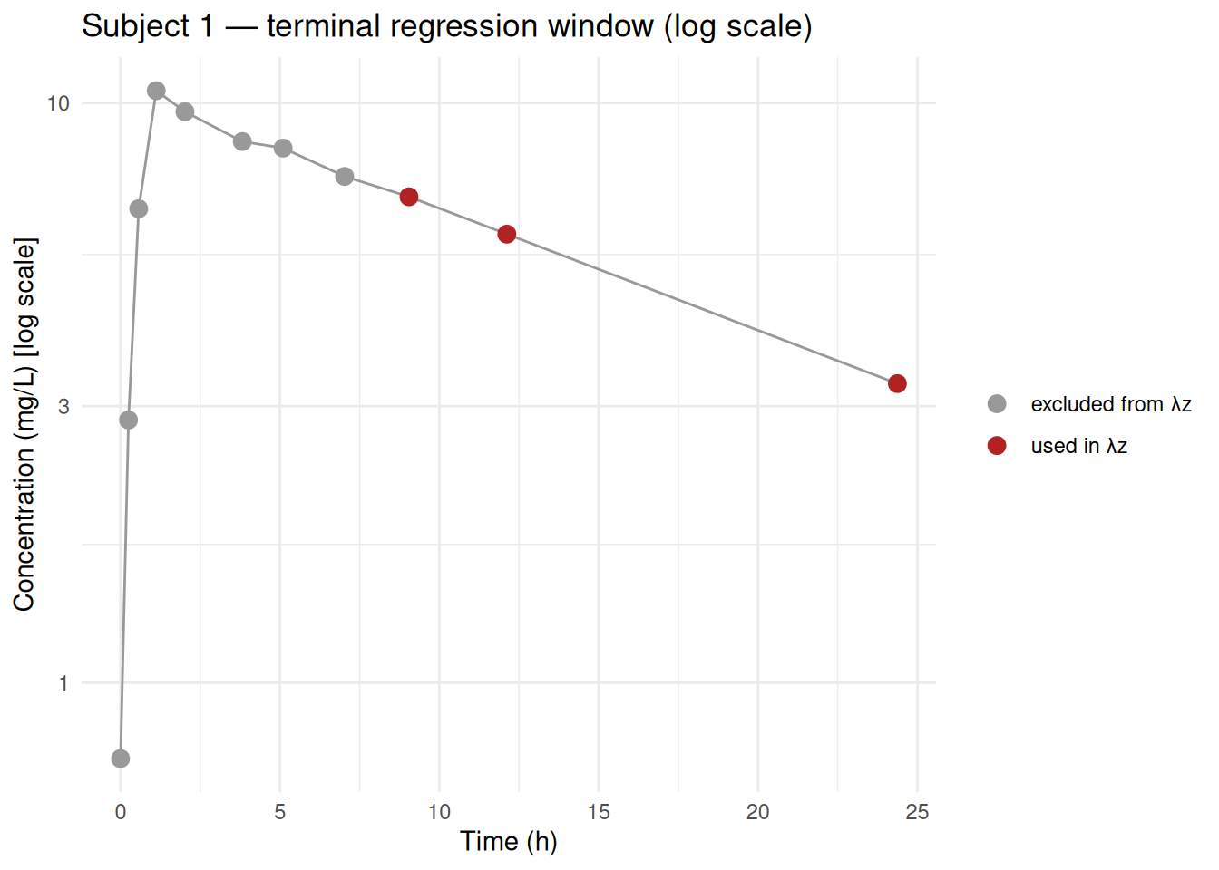
12 5 0.999 0.998 -0.999 8.005.7 Visualising the chosen regression window
# Extract lambda.z.time.first and n.points to annotate the plot
hl_results <- as.data.frame(o_nca) |>
  filter(PPTESTCD %in% c("lambda.z.time.first", "lambda.z.n.points", "tmax")) |>
  tidyr::pivot_wider(names_from = PPTESTCD, values_from = PPORRES)

# Plot subject 1 with regression window highlighted
subj1 <- d_conc |> filter(subject == "1")
win   <- hl_results |> filter(subject == "1")
start_t <- win$lambda.z.time.first

ggplot(subj1, aes(x = time, y = conc)) +
  geom_line(colour = "grey60") +
  geom_point(aes(colour = time >= start_t), size = 3) +
  scale_colour_manual(values = c("FALSE" = "grey60", "TRUE" = "firebrick"),
                      labels = c("excluded from λz", "used in λz"),
                      name = NULL) +
  scale_y_log10() +
  labs(title = "Subject 1 — terminal regression window (log scale)",
       x = "Time (h)", y = "Concentration (mg/L) [log scale]") +
  theme_minimal()