Time to steady state (TSS) is the dosing occasion (or clock time) at which pre-dose trough concentrations are no longer meaningfully rising. PKNCA provides two NCA-based methods for estimating TSS from trough concentration data collected across multiple dose occasions.
Both methods work on trough concentrations (Ctrough = pre-dose concentration) collected at successive dose numbers, not full PK profiles.
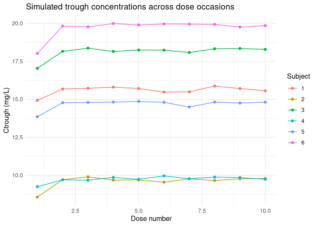
12.2 Simulated dataset
We simulate trough concentrations for 6 subjects across 10 dose occasions. Concentrations approach an individual steady-state plateau following a monoexponential rise.
set.seed(42)n_subjects <-6n_doses <-10d_tss <-data.frame(Subject =rep(1:n_subjects, each = n_doses),dose_number =rep(1:n_doses, n_subjects),ke =rep(0.1*exp(rnorm(n_subjects, 0, 0.2)), each = n_doses),Css =rep(10*exp(rnorm(n_subjects, 0, 0.3)), each = n_doses))d_tss$ctrough <- d_tss$Css * (1-exp(-d_tss$ke * d_tss$dose_number *24)) +rnorm(nrow(d_tss), 0, 0.1)ggplot(d_tss, aes(x = dose_number, y = ctrough, group = Subject, colour =factor(Subject))) +geom_line() +geom_point() +labs(title ="Simulated trough concentrations across dose occasions",x ="Dose number", y ="Ctrough (mg/L)", colour ="Subject") +theme_minimal()
Warning in nlme.formula(conc ~ ctrough.ss * (1 - exp(tss.constant * time/tss)),
: Iteration 1, LME step: nlminb() did not converge (code = 1). Do increase
'msMaxIter'!
Warning in pk.tss.monoexponential.population(modeldata, output =
intersect(c("population", : tss.monoexponential.popind was requested, but the
best model did not include a random effect for tss.  Set to NA.
tss_mono
  subject tss.monoexponential.population tss.monoexponential.popind
1       1                      0.8797774                         NA
2       2                      0.8797774                         NA
3       3                      0.8797774                         NA
4       4                      0.8797774                         NA
5       5                      0.8797774                         NA
6       6                      0.8797774                         NA
  tss.monoexponential.individual tss.monoexponential.single
1                      0.7536625                  0.8806135
2                      1.0731366                  0.8806135
3                      0.8498045                  0.8806135
4                      0.8060571                  0.8806135
5                      0.8277943                  0.8806135
6                      0.9719632                  0.8806135
Interpreting the output columns:
Column
Meaning
tss.monoexponential.population
TSS from population-level fit (one value shared across subjects)
tss.monoexponential.popind
TSS from mixed model with subject-level random effect for TSS (NA if not supported by data)
Warning in nlme.formula(conc ~ ctrough.ss * (1 - exp(tss.constant * time/tss)),
: Iteration 1, LME step: nlminb() did not converge (code = 1). Do increase
'msMaxIter'!
Warning in nlme.formula(conc ~ ctrough.ss * (1 - exp(tss.constant * time/tss)),
: Singular precision matrix in level -1, block 1
Warning in pk.tss.monoexponential.population(modeldata, output =
intersect(c("population", : tss.monoexponential.popind was requested, but the
best model did not include a random effect for tss.  Set to NA.
  subject tss.monoexponential.population tss.monoexponential.popind
1       1                       1.144617                         NA
2       2                       1.144617                         NA
3       3                       1.144617                         NA
4       4                       1.144617                         NA
5       5                       1.144617                         NA
6       6                       1.144617                         NA
  tss.monoexponential.individual tss.monoexponential.single
1                      0.9805283                   1.145705
2                      1.3961661                   1.145705
3                      1.1056088                   1.145705
4                      1.0486509                   1.145705
5                      1.0769848                   1.145705
6                      1.2645547                   1.145705
12.4 Method 2: Stepwise linear (pk.tss.stepwise.linear)
A non-parametric approach: iteratively tests whether concentrations are still increasing linearly from dose occasion \(k\) onward. TSS is the earliest dose occasion at which the upward trend is no longer statistically significant.
This method is more robust when the rise to steady state is irregular or non-monoexponential.
The result is a data frame with a tss.stepwise.linear column containing the first dose occasion number where concentrations are deemed flat (or NA if steady state cannot be determined from the data).
12.5 Combined method (pk.tss)
pk.tss() runs both methods and returns results side by side:
Warning in nlme.formula(conc ~ ctrough.ss * (1 - exp(tss.constant * time/tss)),
: Iteration 1, LME step: nlminb() did not converge (code = 1). Do increase
'msMaxIter'!
Warning in pk.tss.monoexponential.population(modeldata, output =
intersect(c("population", : tss.monoexponential.popind was requested, but the
best model did not include a random effect for tss.  Set to NA.
tss_combined
  subject tss.monoexponential.population tss.monoexponential.popind
1       1                      0.8797774                         NA
2       2                      0.8797774                         NA
3       3                      0.8797774                         NA
4       4                      0.8797774                         NA
5       5                      0.8797774                         NA
6       6                      0.8797774                         NA
  tss.monoexponential.individual tss.monoexponential.single tss.stepwise.linear
1                      0.7536625                  0.8806135                   2
2                      1.0731366                  0.8806135                   2
3                      0.8498045                  0.8806135                   2
4                      0.8060571                  0.8806135                   2
5                      0.8277943                  0.8806135                   2
6                      0.9719632                  0.8806135                   2
12.6 Key arguments
Argument
Default
Meaning
conc
—
Trough concentrations (one per dose occasion per subject)
time
—
Dose occasion numbers or actual clock times
subject
—
Subject identifiers
time.dosing
—
All possible dosing occasions in the study (needed to define the full grid)
tss.fraction
0.9
Fraction of Css that defines “at steady state” (monoexponential method)
output
c("population","popind","individual","single")
Which output types to return
verbose
FALSE
Print model fitting details
Note: TSS estimation requires multiple dose occasions with consistent trough sampling. It is not applicable to single-dose studies or studies where trough collection was inconsistent.
---title: "Time to Steady State"---```{r setup, include=FALSE}library(PKNCA)library(dplyr)library(ggplot2)conflicted::conflicts_prefer(dplyr::filter, dplyr::select, .quiet =TRUE)```## What is time to steady state?**Time to steady state (TSS)** is the dosing occasion (or clock time) at which pre-dose trough concentrations are no longer meaningfully rising. PKNCA provides two NCA-based methods for estimating TSS from trough concentration data collected across multiple dose occasions.Both methods work on trough concentrations (Ctrough = pre-dose concentration) collected at successive dose numbers, not full PK profiles.---## Simulated datasetWe simulate trough concentrations for 6 subjects across 10 dose occasions. Concentrations approach an individual steady-state plateau following a monoexponential rise.```{r}set.seed(42)n_subjects <-6n_doses <-10d_tss <-data.frame(Subject =rep(1:n_subjects, each = n_doses),dose_number =rep(1:n_doses, n_subjects),ke =rep(0.1*exp(rnorm(n_subjects, 0, 0.2)), each = n_doses),Css =rep(10*exp(rnorm(n_subjects, 0, 0.3)), each = n_doses))d_tss$ctrough <- d_tss$Css * (1-exp(-d_tss$ke * d_tss$dose_number *24)) +rnorm(nrow(d_tss), 0, 0.1)ggplot(d_tss, aes(x = dose_number, y = ctrough, group = Subject, colour =factor(Subject))) +geom_line() +geom_point() +labs(title ="Simulated trough concentrations across dose occasions",x ="Dose number", y ="Ctrough (mg/L)", colour ="Subject") +theme_minimal()```---## Method 1: Monoexponential (`pk.tss.monoexponential`)Fits a monoexponential approach-to-plateau model:$$C_{\text{trough}}(n) = C_{ss} \cdot \left(1 - e^{-k_{\text{tss}} \cdot n}\right)$$Reports TSS as the dose occasion at which the predicted concentration reaches a specified fraction of Css (default: 90% = `tss.fraction = 0.9`).Returns population, population-individual (popind), individual, and single-subject estimates.```{r}tss_mono <-pk.tss.monoexponential(conc = d_tss$ctrough,time = d_tss$dose_number,subject = d_tss$Subject,time.dosing =1:n_doses)tss_mono```**Interpreting the output columns:**| Column | Meaning ||---|---||`tss.monoexponential.population`| TSS from population-level fit (one value shared across subjects) ||`tss.monoexponential.popind`| TSS from mixed model with subject-level random effect for TSS (NA if not supported by data) ||`tss.monoexponential.individual`| TSS from individual-level fits ||`tss.monoexponential.single`| TSS ignoring between-subject variability |### Changing the fraction threshold```{r}# 95% of Csspk.tss.monoexponential(conc = d_tss$ctrough,time = d_tss$dose_number,subject = d_tss$Subject,time.dosing =1:n_doses,tss.fraction =0.95)```---## Method 2: Stepwise linear (`pk.tss.stepwise.linear`)A non-parametric approach: iteratively tests whether concentrations are still increasing linearly from dose occasion $k$ onward. TSS is the earliest dose occasion at which the upward trend is no longer statistically significant.This method is more robust when the rise to steady state is irregular or non-monoexponential.```{r}tss_linear <-pk.tss.stepwise.linear(conc = d_tss$ctrough,time = d_tss$dose_number,subject = d_tss$Subject,time.dosing =1:n_doses)tss_linear```The result is a data frame with a `tss.stepwise.linear` column containing the first dose occasion number where concentrations are deemed flat (or `NA` if steady state cannot be determined from the data).---## Combined method (`pk.tss`)`pk.tss()` runs both methods and returns results side by side:```{r}tss_combined <-pk.tss(conc = d_tss$ctrough,time = d_tss$dose_number,subject = d_tss$Subject,time.dosing =1:n_doses)tss_combined```---## Key arguments| Argument | Default | Meaning ||---|---|---||`conc`| — | Trough concentrations (one per dose occasion per subject) ||`time`| — | Dose occasion numbers or actual clock times ||`subject`| — | Subject identifiers ||`time.dosing`| — | All possible dosing occasions in the study (needed to define the full grid) ||`tss.fraction`|`0.9`| Fraction of Css that defines "at steady state" (monoexponential method) ||`output`|`c("population","popind","individual","single")`| Which output types to return ||`verbose`|`FALSE`| Print model fitting details |> **Note:** TSS estimation requires **multiple dose occasions with consistent trough sampling**. It is not applicable to single-dose studies or studies where trough collection was inconsistent.---::: {.callout-note icon=false appearance="minimal"}**pkgdown reference:** [pk.tss()](https://humanpred.github.io/pknca/reference/pk.tss.html) · [pk.tss.monoexponential()](https://humanpred.github.io/pknca/reference/pk.tss.monoexponential.html) · [pk.tss.stepwise.linear()](https://humanpred.github.io/pknca/reference/pk.tss.stepwise.linear.html):::