flowchart LR
    A["AUClast\n0 → last measurable"]
    B["AUCall\n0 → last, zeros for BLQ"]
    C["AUCinf.obs\n0 → ∞ (observed Clast)"]
    D["AUCinf.pred\n0 → ∞ (predicted Clast)"]
    E["AUCint / partial\n0 → t (any t)"]
4 AUC Types and Integration Methods
4.1 AUC types
PKNCA offers four families of AUC, each answering a different question:
| Parameter | End point | BLQ treatment | When to use |
|---|---|---|---|
auclast |
Last measurable concentration | BLQs after last non-BLQ are ignored | Default; most studies |
aucall |
Last measured time point | Post-last-measurable BLQs treated as 0 | When you want to include the BLQ tail |
aucinf.obs |
Extrapolated to ∞ (using observed Clast) | — | When half-life is reliable |
aucinf.pred |
Extrapolated to ∞ (using predicted Clast from λz fit) | — | When Clast is noisy |
aucint.* |
Any user-defined time window | — | Partial AUC, bioequivalence |
4.1.1 AUClast vs AUCall
auc_compare <- data.frame(
  start    = 0,
  end      = Inf,
  auclast  = TRUE,
  aucall   = TRUE,
  aucinf.obs = TRUE
)

o_data <- PKNCAdata(o_conc, o_dose, intervals = auc_compare)
o_nca  <- pk.nca(o_data)

as.data.frame(o_nca) |>
  filter(PPTESTCD %in% c("auclast", "aucall", "aucinf.obs", "aucpext.obs")) |>
  select(PPTESTCD, PPORRES)
# A tibble: 3 × 2
PPTESTCD PPORRES
<chr> <dbl>
1 auclast 147.
2 aucall 147.
3 aucinf.obs 215.
aucall≥auclastwhen there are post-last-measurable BLQ timepoints, since those are treated as 0 and add a small triangle to the AUC.
4.2 Partial AUC (AUCint)
For bioequivalence or exposure-in-a-window calculations, use aucint.* parameters. These calculate AUC over an exact time window, interpolating concentrations at the boundaries if needed.
# AUC from 0 to 4h and 0 to 12h on the same profile
partial_intervals <- data.frame(
  start         = c(0,  0),
  end           = c(4, 12),
  aucint.last   = TRUE,   # AUC to the last obs within window (or interpolated boundary)
  aucint.inf.obs = FALSE
)

o_data_partial <- PKNCAdata(o_conc, o_dose, intervals = partial_intervals)
o_nca_partial  <- pk.nca(o_data_partial)

as.data.frame(o_nca_partial) |>
  filter(PPTESTCD == "aucint.last") |>
  select(start, end, PPTESTCD, PPORRES)
# A tibble: 2 × 4
start end PPTESTCD PPORRES
<dbl> <dbl> <chr> <dbl>
1 0 4 aucint.last 33.7
2 0 12 aucint.last 91.7All partial AUC variants:
| Parameter | End concentration | Dose-aware boundary | Extrapolation |
|---|---|---|---|
aucint.last |
Last observed in window | No | None |
aucint.all |
Last observed, BLQs as 0 | No | None |
aucint.inf.obs |
Extrapolated to ∞, observed Clast | No | λz-based tail |
aucint.inf.pred |
Extrapolated to ∞, predicted Clast | No | λz-based tail |
aucint.last.dose |
Same as .last |
Yes | None |
aucint.all.dose |
Same as .all |
Yes | None |
aucint.inf.obs.dose |
Same as .inf.obs |
Yes | λz-based tail |
aucint.inf.pred.dose |
Same as .inf.pred |
Yes | λz-based tail |
Note:
aucint.inf.predrequires thatlambda.zhas been estimated (i.e., that the terminal slope is calculable from the data window).
The .dose variants use dose-aware interpolation (interp.extrap.conc.dose()) at the interval start and end. This matters when the interval boundary coincides with a dose time — the .dose variant correctly handles the before/after concentration jump.
# All partial AUC variants over a single window
all_partial <- data.frame(
  start                 = 0,
  end                   = 8,
  aucint.last           = TRUE,
  aucint.all            = TRUE,
  aucint.inf.obs        = TRUE,
  aucint.inf.pred       = TRUE,
  aucint.last.dose      = TRUE,
  aucint.all.dose       = TRUE,
  aucint.inf.obs.dose   = TRUE,
  aucint.inf.pred.dose  = TRUE
)

o_nca_all_partial <- pk.nca(PKNCAdata(o_conc, o_dose, intervals = all_partial))
as.data.frame(o_nca_all_partial) |>
  filter(grepl("^aucint", PPTESTCD)) |>
  select(PPTESTCD, PPORRES)
# A tibble: 8 × 2
PPTESTCD PPORRES
<chr> <dbl>
1 aucint.last 65.3
2 aucint.last.dose 65.3
3 aucint.all 65.3
4 aucint.all.dose 65.3
5 aucint.inf.obs 65.3
6 aucint.inf.obs.dose 65.3
7 aucint.inf.pred 65.3
8 aucint.inf.pred.dose 65.34.3 Percent extrapolation (%AUCextrap)
When using aucinf, you should check what fraction was extrapolated beyond the last observation. A high aucpext means the terminal phase was poorly characterised.
pext_interval <- data.frame(
  start        = 0,
  end          = Inf,
  auclast      = TRUE,
  aucinf.obs   = TRUE,
  aucpext.obs  = TRUE,
  aucpext.pred = TRUE
)

o_nca_pext <- pk.nca(PKNCAdata(o_conc, o_dose, intervals = pext_interval))
as.data.frame(o_nca_pext) |>
  filter(grepl("^auc", PPTESTCD)) |>
  select(PPTESTCD, PPORRES)
# A tibble: 5 × 2
PPTESTCD PPORRES
<chr> <dbl>
1 auclast 147.
2 aucinf.obs 215.
3 aucinf.pred 215.
4 aucpext.obs 31.5
5 aucpext.pred 31.5The default threshold is max.aucinf.pext = 20 (%). Results where aucpext > 20% are flagged with an exclude message. Change the threshold via options:
# Stricter: flag if more than 10% is extrapolated
o_data_strict <- PKNCAdata(o_conc, o_dose, intervals = pext_interval,
                            options = list(max.aucinf.pext = 10))
o_nca_strict  <- pk.nca(o_data_strict)
as.data.frame(o_nca_strict) |>
  filter(PPTESTCD == "aucinf.obs") |>
  select(PPTESTCD, PPORRES, exclude)
# A tibble: 1 × 3
PPTESTCD PPORRES exclude
<chr> <dbl> <chr>
1 aucinf.obs 215. <NA> 4.4 Integration methods
The integration method controls how the area of each trapezoid is computed between consecutive timepoints.
# Visual comparison of the three methods on one subject
methods <- c("linear", "lin-log", "lin up/log down")

results <- lapply(methods, function(m) {
  o <- pk.nca(PKNCAdata(o_conc, o_dose,
                        intervals = data.frame(start=0, end=Inf, auclast=TRUE),
                        options   = list(auc.method = m)))
  as.data.frame(o) |>
    filter(PPTESTCD == "auclast") |>
    mutate(method = m)
}) |> bind_rows()

results |> select(method, PPORRES) |>
  rename(auclast = PPORRES)
# A tibble: 3 × 2
method auclast
<chr> <dbl>
1 linear 149.
2 lin-log 147.
3 lin up/log down 147.4.4.1 Method details
Linear trapezoidal ("linear")
Uses the standard trapezoidal rule throughout: \[\text{AUC}_{t_i \to t_{i+1}} = \frac{(C_i + C_{i+1})}{2} \times (t_{i+1} - t_i)\]
Overestimates during the descending phase (gives too much weight to the higher concentration).
Lin-log ("lin-log")
Uses linear integration from start up to Tmax, and log-linear integration from Tmax onward: \[\text{AUC}_{t_i \to t_{i+1}} = \frac{(C_i - C_{i+1})}{\ln C_i - \ln C_{i+1}} \times (t_{i+1} - t_i) \quad \text{(post-Tmax)}\]
The switch point is Tmax (not whether concentrations are rising or falling), so any post-Tmax secondary peak is integrated log-linearly even if concentrations are rising. Falls back to linear for any interval where either endpoint is zero. Not recommended — "lin up/log down" is strictly better for nearly all use cases as it switches on actual direction rather than Tmax.
Lin up / log down ("lin up/log down") — default
Hybrid: linear trapezoidal on the ascending phase (when \(C_{i+1} \geq C_i\)), log-linear on the descending phase (when \(C_{i+1} < C_i\)). Best of both worlds for most PK profiles.
# Visualise the three profiles for one subject
d_plot <- d_one |>
  filter(conc > 0) |>
  arrange(time)

# Illustrate the interpolated concentration between two points
t_seq <- seq(min(d_plot$time), max(d_plot$time), length.out = 200)

ggplot(d_plot, aes(x = time, y = conc)) +
  geom_line(colour = "steelblue", linewidth = 1) +
  geom_point(size = 3, colour = "steelblue") +
  geom_area(alpha = 0.15, fill = "steelblue") +
  labs(title = "Concentration-time profile (shaded area = AUClast)",
       x = "Time (h)", y = "Concentration (mg/L)") +
  theme_minimal()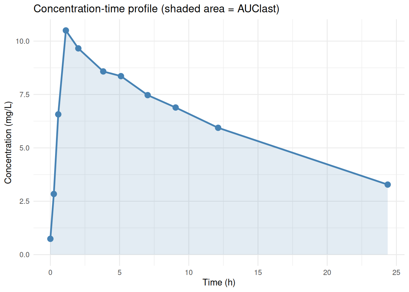
4.4.2 When to use which method
| Study type | Recommended method | Notes |
|---|---|---|
| Most oral/extravascular | "lin up/log down" (default) |
Linear on ascending phase, log-linear on declining phase |
| IV bolus | "lin up/log down" (default) |
Profile is entirely declining, so log-linear is used throughout — equivalent to "lin-log" for pure bolus but without the Tmax ambiguity |
| IV infusion with smooth decline | "lin up/log down" |
Concentrations rise during infusion (linear) then fall after end of infusion (log-linear) |
| Regulatory (some agencies) | "linear" |
Some health authorities require the linear trapezoidal rule throughout |
| Highly irregular profiles with zeros | "linear" |
Log-linear is undefined when either endpoint is zero; "linear" is the safe fallback |
| Never recommended | "lin-log" |
Switches at Tmax rather than on direction of change — gives wrong method for post-Tmax secondary peaks |
4.5 AUMC — area under the first moment curve
The AUMC is used to compute MRT. It weights concentrations by time: \[\text{AUMC} = \int_0^{t} t \cdot C(t) \, dt\]
aumc_interval <- data.frame(
  start        = 0,
  end          = Inf,
  aumclast     = TRUE,
  aumcinf.obs  = TRUE
)

o_nca_aumc <- pk.nca(PKNCAdata(o_conc, o_dose, intervals = aumc_interval))
as.data.frame(o_nca_aumc) |>
  filter(grepl("^aumc", PPTESTCD)) |>
  select(PPTESTCD, PPORRES)
# A tibble: 2 × 2
PPTESTCD PPORRES
<chr> <dbl>
1 aumclast 1499.
2 aumcinf.obs 4546.4.6 AUC above a threshold (aucabove.*)
aucabove.* computes the area under the curve above a reference concentration — useful for quantifying time above a minimum effective concentration or below a toxicity threshold.
| Parameter | Reference concentration |
|---|---|
aucabove.trough.all |
Ctrough (concentration at end of interval) |
aucabove.predose.all |
Cpredose (concentration at interval start) |
above_interval <- data.frame(
  start              = 0,
  end                = 24,
  aucabove.trough.all  = TRUE,
  aucabove.predose.all = TRUE,
  ctrough              = TRUE,
  cstart               = TRUE
)

o_nca_above <- pk.nca(PKNCAdata(o_conc, o_dose, intervals = above_interval))

as.data.frame(o_nca_above) |>
  filter(PPTESTCD %in% c("aucabove.trough.all", "aucabove.predose.all", "ctrough", "cstart")) |>
  select(PPTESTCD, PPORRES)
# A tibble: 4 × 2
PPTESTCD PPORRES
<chr> <dbl>
1 ctrough NA
2 cstart 0.74
3 aucabove.predose.all 83.4
4 aucabove.trough.all NA 4.7 Time above a threshold (time_above)
time_above computes the total duration (in time units) for which the concentration exceeds a specified threshold. The threshold is set via the conc_above column in the intervals data frame.
# Time above 2 mg/L
time_above_interval <- data.frame(
  start      = 0,
  end        = Inf,
  time_above = TRUE,
  conc_above = 2       # threshold concentration (same units as your data)
)

o_nca_ta <- pk.nca(PKNCAdata(o_conc, o_dose, intervals = time_above_interval))

as.data.frame(o_nca_ta) |>
  filter(PPTESTCD == "time_above") |>
  select(PPTESTCD, PPORRES)
# A tibble: 1 × 2
PPTESTCD PPORRES
<chr> <dbl>
1 time_above 24.24.8 Total dose (totdose)
totdose is the total amount administered within the analysis interval — it is extracted from the dose object rather than computed from concentrations. Useful as a reference column in your results data frame.
totdose_interval <- data.frame(
  start    = 0,
  end      = Inf,
  totdose  = TRUE,
  auclast  = TRUE
)

o_nca_td <- pk.nca(PKNCAdata(o_conc, o_dose, intervals = totdose_interval))

as.data.frame(o_nca_td) |>
  filter(PPTESTCD %in% c("totdose", "auclast")) |>
  select(PPTESTCD, PPORRES)
# A tibble: 2 × 2
PPTESTCD PPORRES
<chr> <dbl>
1 auclast 147.
2 totdose 320.4.9 AUMC variants
The area under the first-moment curve (AUMC) is used to calculate MRT.
| Parameter | Meaning |
|---|---|
aumclast |
AUMC from 0 to last measurable concentration |
aumcall |
AUMC from 0 to last, treating BLQ as 0 |
aumcinf.obs |
AUMC extrapolated to ∞, observed Clast |
aumcinf.pred |
AUMC extrapolated to ∞, predicted Clast |
aumc_interval <- data.frame(
  start         = 0,
  end           = Inf,
  aumclast      = TRUE,
  aumcall       = TRUE,
  aumcinf.obs   = TRUE,
  aumcinf.pred  = TRUE
)

o_nca_aumc <- pk.nca(PKNCAdata(o_conc, o_dose, intervals = aumc_interval))

as.data.frame(o_nca_aumc) |>
  filter(grepl("^aumc", PPTESTCD)) |>
  select(PPTESTCD, PPORRES)
# A tibble: 4 × 2
PPTESTCD PPORRES
<chr> <dbl>
1 aumclast 1499.
2 aumcall 1499.
3 aumcinf.obs 4546.
4 aumcinf.pred 4546.4.10 Cav over a specific interval (cav.int.*)
cav.int.* computes the average concentration over a specified window using the trapezoidal rule, without requiring a full dosing-interval design.
| Parameter | Window |
|---|---|
cav.int.last |
0 to last measurable |
cav.int.all |
0 to last, BLQ = 0 |
cav.int.inf.obs |
0 to ∞, observed Clast |
cav.int.inf.pred |
0 to ∞, predicted Clast |
cav_interval <- data.frame(
  start             = 0,
  end               = Inf,
  cav.int.last      = TRUE,
  cav.int.all       = TRUE,
  cav.int.inf.obs   = TRUE,
  cav.int.inf.pred  = TRUE
)

o_nca_cav <- pk.nca(PKNCAdata(o_conc, o_dose, intervals = cav_interval))

as.data.frame(o_nca_cav) |>
  filter(grepl("^cav.int", PPTESTCD)) |>
  select(PPTESTCD, PPORRES)
# A tibble: 4 × 2
PPTESTCD PPORRES
<chr> <dbl>
1 cav.int.last 0
2 cav.int.all 0
3 cav.int.inf.obs 0
4 cav.int.inf.pred 04.11 Concentration interpolation at interval boundaries
When a requested interval boundary (e.g., end = 8) falls between two observed timepoints, PKNCA interpolates the concentration at that boundary before computing AUC.
The interpolation method matches the AUC method: - "linear" → linear interpolation - "lin up/log down" → log-linear interpolation on the descending phase
# end=5h falls between t=4 and t=7.02 in the Theoph dataset
interp_interval <- data.frame(start = 0, end = 5, auclast = TRUE)
o_nca_interp <- pk.nca(PKNCAdata(o_conc, o_dose, intervals = interp_interval))
as.data.frame(o_nca_interp) |>
  filter(PPTESTCD == "auclast") |>
  select(start, end, PPTESTCD, PPORRES)
# A tibble: 1 × 4
start end PPTESTCD PPORRES
<dbl> <dbl> <chr> <dbl>
1 0 5 auclast 32.1