PKNCA Training Sessions

Introduction to PKNCA and Basics of Its Use

Creation of these materials were partially supported by funding from the Metrum Research Group.

Introduction to PKNCA

PKNCA is a tool for calculating noncompartmental analysis (NCA) results for pharmacokinetic (PK) data.

… but, you already knew that or you wouldn’t be here.

PKNCA has several foci:

be regulatory-ready
- it has approximately 100% test coverage.
be reproducible
- it has a focus on being scriptable.
get the right answer or none at all
- it will try to know what you want,
- but all decisions can be overridden, and
- if there is a question that may cause an error or an unanticipated result, either no result will output or an error will be raised.

Enjoy!

I hope that you have a whale of a good time during this training.

(Foreshadowing…)

Some NCA Definitions

C_max: The maximum observed concentration
T_max: The time of the maximum observed concentration
t_last: The time of the last concentration above the limit of quantification
AUC: Area under the concentration-time curve. Some important AUC variants are:
- AUC_last: AUC from time zero to t_last
- AUC_int: AUC from time zero to the end of an interval of time, often extrapolated or interpolated (e.g. AUC_0-24hr)
- AUC_∞: AUC from time zero to t_last then extrapolated from t_last to time infinity using the half life

Dataset Basics

NCA Data are Not Tidy as a Single Dataset

“Tidy datasets… have a specific structure: each variable is a column, each observation is a row, and each type of observational unit is a table.” - Hadley Wickham (https://doi.org/10.18637/jss.v059.i10)

CDISC has NCA tidied, and PKNCA follows that model:

concentration-time is a dataset (PC domain; PKNCAconc() object)
dose-time is a dataset (EX/EC domains; PKNCAdose() object)
NCA results are a dataset (PP domain; pk.nca() output)

Dataset Basics: Minimum data

PKNCA requires at least the concentration, time, and what you want to calculate.

Dataset Basics: What columns are needed?

Column names are provided by the input to PKNCAconc() and PKNCAdose(); they are not hard-coded.

Columns that can be used include:

PKNCAconc(): concentration, time, groups; data exclusions; half-life inclusion and exclusion
PKNCAdose(): dose, time, groups; route, rate/duration of infusion; data exclusions
intervals given to PKNCAdata(): groups, start, end, and any NCA parameters to calculate

Dataset Basics: Example data

In the following slides, abbreviated data from an example study where two treatments (“A” and “B”) are administered to two subjects (1 and 2).

For PKNCA, the groups will be Treatment and Subject.
- PKNCA considers groups in order with the subject identifier as the last group (or the last group before a forward slash, /, if / is present).
- When indicated in order (...|Treatment+Subject), PKNCA automatically knows to keep Treatment and drop Subject for summaries (more on that later).

Dataset Basics: Example concentration data

Subject	Treatment	Time	Conc
1	A	0	0
1	A	2	2.143
1	A	8	0.4696
1	B	0	0
1	B	2	2.179
1	B	8	0.4852

Subject	Treatment	Time	Conc
2	A	0	0
2	A	2	1.937
2	A	8	0.4929
2	B	0	0
2	B	2	2.127
2	B	8	0.4804

Dataset Basics: Example dosing data

Subject	Treatment	Time	Dose
1	A	0	10
1	B	0	10

Subject	Treatment	Time	Dose
2	A	0	10
2	B	0	10

Dataset Basics: Example interval data

d_interval_1 <-
  data.frame(
    start=0, end=8,
    cmax=TRUE, tmax=TRUE, auclast=TRUE
  )

start	end	cmax	tmax	auclast
0	8	TRUE	TRUE	TRUE

Groups are not required, if you want the same intervals calculated for each group.

Hands-on: First NCA calculation with PKNCA

library(dplyr)
library(ggplot2)
library(tidyr)
library(purrr)
library(PKNCA)
# Concentration data setup
d_conc <-
  datasets::Theoph %>%
  filter(Subject %in% 1)
o_conc <- PKNCAconc(conc~Time, data=d_conc)
# Setup intervals for calculation
d_intervals <- data.frame(start=0, end=24, cmax=TRUE, tmax=TRUE,
                          auclast=TRUE, aucint.inf.obs=TRUE)
# Combine concentration and dose
o_data <- PKNCAdata(o_conc, intervals=d_intervals)
# Calculate the results (suppressMessages() hides a message that isn't needed now)
o_result <- suppressMessages(pk.nca(o_data))
# summary(o_result)

PKNCA Functions

What functions are the most used?

PKNCAconc(): define a concentration-time PKNCAconc object
- All information about concentration data are given: concentration, time
- Optional information includes: grouping information (usually given), data to exclude, half-life inclusion and exclusion columns
PKNCAdose(): define a dose-time PKNCAdose object (optional)
- dose amount and time are both optional
- Optional information includes: rate or duration of infusion, data to exclude
PKNCAdata(): combine PKNCAconc, optionally PKNCAdose, and optionally intervals into a PKNCAdata object
- the PKNCAconc object must be given; the PKNCAdose object is optional; interval definitions are usually given; calculation options may be given
pk.nca(): calculate the NCA parameters from a data object into a PKNCAresults object

How do I do a simple calculation? all steps

We will break this down in subsequent slides.

# Concentration data setup
d_conc <-
  datasets::Theoph %>%
  filter(Subject %in% 1)
o_conc <- PKNCAconc(conc~Time, data=d_conc)
# Dose data setup
d_dose <-
  datasets::Theoph %>%
  filter(Subject %in% 1) %>%
  filter(Time == 0)
o_dose <- PKNCAdose(Dose~Time, data=d_dose)
# Combine concentration and dose
o_data <- PKNCAdata(o_conc, o_dose)
# Calculate the results
o_result <- pk.nca(o_data)

How do I do a simple calculation? Concentration data

# Load your dataset as a data.frame
d_conc <-
  datasets::Theoph %>%
  filter(Subject %in% 1)
# Take a look at the data
pander::pander(head(d_conc, 2))

Subject	Wt	Dose	Time	conc
1	79.6	4.02	0	0.74
1	79.6	4.02	0.25	2.84

# Define the PKNCAconc object indicating the concentration and time columns, the
# dataset, and any other options.
o_conc <- PKNCAconc(conc~Time, data=d_conc)

How do I do a simple calculation? Dose data

# Load your dataset as a data.frame
d_dose <-
  datasets::Theoph %>%
  filter(Subject %in% 1) %>%
  filter(Time == 0)
# Take a look at the data
pander::pander(d_dose)

Subject	Wt	Dose	Time	conc
1	79.6	4.02	0	0.74

# Define the PKNCAdose object indicating the dose amount and time columns, the
# dataset, and any other options.
o_dose <- PKNCAdose(Dose~Time, data=d_dose)

How do I do a simple calculation? Calculate results

# Combine the PKNCAconc and PKNCAdose objects.  You can add interval
# specifications and calculation options here.
o_data <- PKNCAdata(o_conc, o_dose)
# Calculate the results
o_result <- pk.nca(o_data)

How do I do a simple calculation? Get results

To calculate summary statistics, use summary(); to extract all individual-level results, use as.data.frame().

The "caption" attribute of the summary describes how the summary statistics were calculated for each parameter. (Hint: pander::pander() knows how to use that to put the caption on a table in a report.)

The individual results contain the columns for start time, end time, grouping variables (none in this example), parameter names, values, and if the value should be excluded.

How do I do a simple calculation? Get summary results

# Look at summarized results
pander::pander(summary(o_result))

auclast, cmax, aucinf.obs, cl.inf.obs: geometric mean and geometric coefficient of variation; tmax, tlag, count.conc: median and range; half.life, aucpext.inf.obs: arithmetic mean and standard deviation (continued below)
start	end	auclast	cmax	tmax	tlag	count.conc	half.life
0	Inf	147	10.5	1.12	0.000	11.0	14.3

aucinf.obs	aucpext.inf.obs	cl.inf.obs
215	31.5	0.0187

How do I do a simple calculation? Get individual results

Use as.data.frame() to get the individual NCA parameter results.

# Look at individual results
pander::pander(head(
  as.data.frame(o_result),
  n=3
))

end	PPTESTCD	PPORRES	PPANMETH	exclude
Inf	auclast	147.2	Imputation: start_predose_conc0. AUC: lin up/log down	NA
Inf	cmax	10.5	Imputation: start_predose_conc0	NA
Inf	tmax	1.12	Imputation: start_predose_conc0	NA

PKNCA datasets

How does PKNCA think about data?

Three types of data are inputs for calculation in PKNCA:

concentration-time (PKNCAconc),
dose-time (PKNCAdose), and
intervals.

PKNCAconc and PKNCAdose objects can optionally have groups. The groups in a PKNCAdose object must be the same or fewer than the groups in PKNCAconc object (for example, all subjects in a treatment arm may receive the same dose).

What is an “interval” and how is it different than a “group”?

A group separates one full concentration-time profile for a subject that you may ever want to consider at the same time. Usually, it groups by study, treatment, analyte, and subject (other groups can be useful depending on the study design).

An interval selects a time range within a group.

One time can be in zero or more intervals, but only zero or one group. Intervals can be adjacent (0-12 and 12-24) or overlap (0-12 and 0-24). In other words, one sample may be used in more than one interval, but one sample will never be used in more than one group.

Legend: The group contains all points on the figure. Shaded regions indicate intervals. Arrows indicate points shared between intervals within the group.

Common data management requirements before sending data to PKNCA

Time must not be missing for PKNCAconc (if given to PKNCAdose, it must not be missing).
Below the limit of quantification (BLQ) concentrations must be set to zero (not NA).
Imputation of time zero is required for AUC calculation.
Especially for actual-time calculations, imputation of the beginning of the interval is usually needed.

Columns must be created for:

Concentration or dose,
Time
Groups
- usually columns for study, treatment arm, subject;
- sometimes analyte, formulation, period (needed in case the same subject receives the same treatment arm multiple times)

Setup your concentration data

Concentration data must be numeric

Setup your concentration data

Concentration data must be numeric
Time must be numeric and not be missing

Setup your concentration data

Concentration data must be numeric
Time must be numeric and not be missing
Groups can be anything, setup at the level of the individual

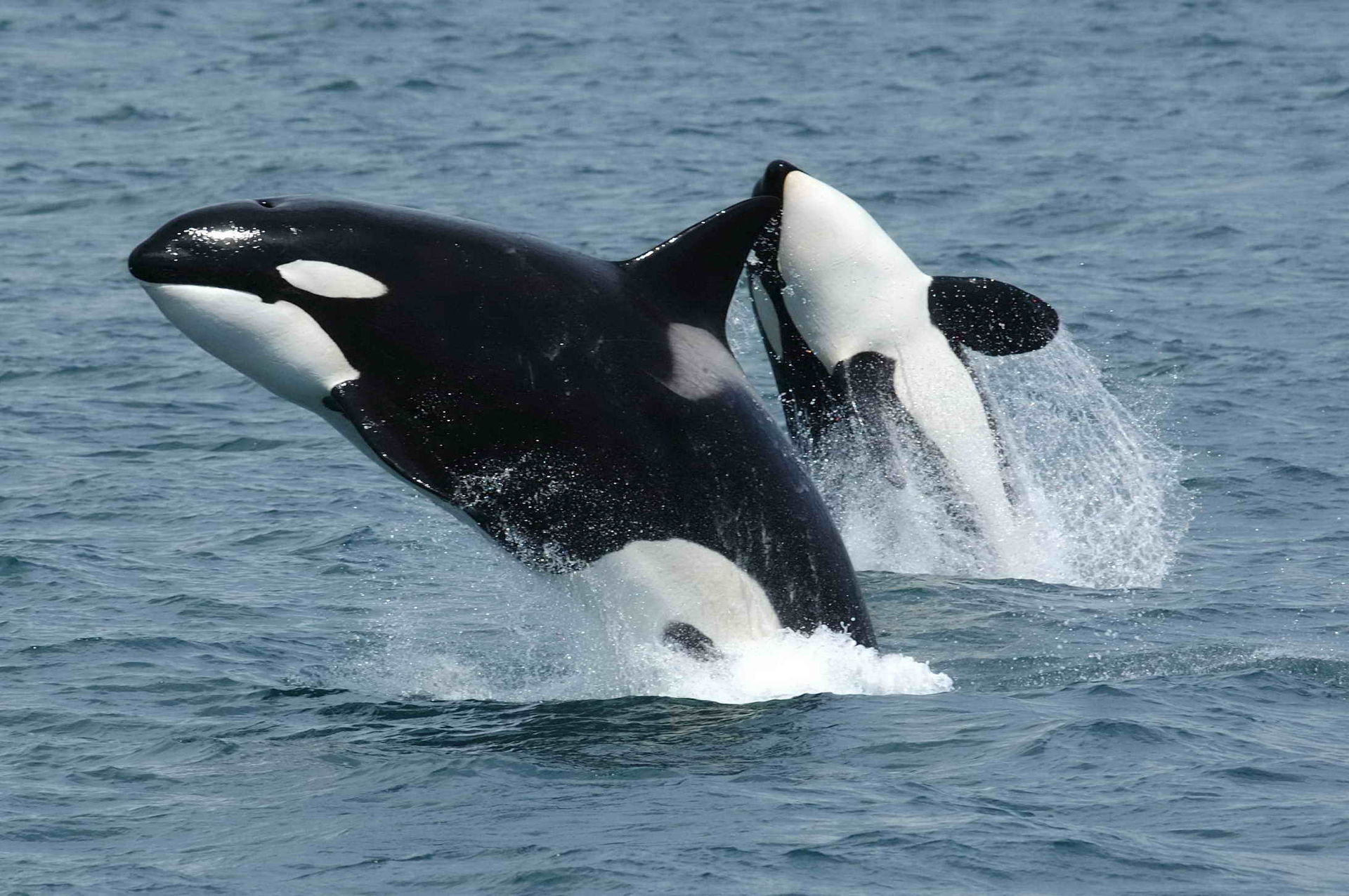
Group: 🗸 a pod of killer whales

Setup your dosing data (if you have it and even if you don’t)

Normal dosing data setup: PKNCAdose(dose~time|actarm+usubjid, data=d_dose)

Dose amount must be numeric — or it can be omitted
- PKNCAdose(~time|actarm+usubjid, data=d_dose)
Time must be numeric and not be missing — or it can be omitted
- PKNCAdose(dose~.|actarm+usubjid, data=d_dose)
Groups can be anything — may be grouped at a higher level than the individual
- Useful when all dose amounts and times are the same within an arm: PKNCAdose(dose~time|actarm, data=d_dose)
- Useful dose amount is the same at all times within an arm: PKNCAdose(dose~.|actarm, data=d_dose)
- Useful when times are all the same within an arm but dose may differ: PKNCAdose(~time|actarm, data=d_dose)

Define your intervals

Intervals have columns for:

start and end times for the interval,
groups matching any level of grouping; intervals apply by a merge/join with the groups
parameters to calculate (TRUE means to calculate it; FALSE means don’t). The full list of available parameters is in the selection of calculation intervals vignette.
- You only have to specify the parameter you want, not all parameters.

Define your intervals: example

For time 0 to 24, calculate AUClast
For time 0 to infinity, calculate cmax, tmax, half.life, and aucinf.obs

start	end	auclast	cmax	tmax	half.life	aucinf.obs
0	24	TRUE	FALSE	FALSE	FALSE	FALSE
0	Inf	FALSE	TRUE	TRUE	TRUE	TRUE

Calculations above the hood

Prepare your data for calculation

d_conc <-
  datasets::Theoph %>%
  mutate(
    Treatment=
      case_when(
        Dose <= median(Dose)~"Low dose",
        TRUE~"High dose"
      )
  )
# The study was single-dose
d_dose <-
  d_conc %>%
  select(Treatment, Subject, Dose) %>%
  unique() %>%
  mutate(dose_time=0)

Calculate without dosing data

o_conc <- PKNCAconc(conc~Time|Treatment+Subject, data=d_conc)
try({
  o_data <- PKNCAdata(o_conc)
  summary(pk.nca(o_data))
})

## Error in PKNCAdata.default(data.conc = data.conc, data.dose = data.dose,  : 
##   If data.dose is not given, intervals must be given

Whoops! Without dosing, we need intervals.

Calculate without dosing data, try 2

o_conc <- PKNCAconc(conc~Time|Treatment+Subject, data=d_conc)
d_intervals <- data.frame(start=0, end=Inf, cmax=TRUE, tmax=TRUE,
                          half.life=TRUE, aucinf.obs=TRUE)
o_data_manual_intervals <- PKNCAdata(o_conc, intervals=d_intervals)
summary(pk.nca(o_data_manual_intervals))

##  start end Treatment N        cmax               tmax   half.life aucinf.obs
##      0 Inf High dose 5 9.16 [19.4] 3.48 [0.980, 3.55] 7.73 [1.08] 120 [26.2]
##      0 Inf  Low dose 7 8.30 [15.2] 1.12 [0.630, 2.02] 8.50 [2.67] 111 [31.6]
## 
## Caption: cmax, aucinf.obs: geometric mean and geometric coefficient of variation; tmax: median and range; half.life: arithmetic mean and standard deviation; N: number of subjects

Dosing data helps with interval setup

o_conc <- PKNCAconc(conc~Time|Treatment+Subject, data=d_conc)
o_dose <- PKNCAdose(Dose~dose_time|Treatment+Subject, data=d_dose)
o_data_auto_intervals <- PKNCAdata(o_conc, o_dose)
o_data_auto_intervals$intervals$aucall <- TRUE
summary(pk.nca(o_data_auto_intervals))

##  start end Treatment N     auclast      aucall        cmax               tmax
##      0 Inf  Low dose 7 94.5 [22.8] 94.5 [22.8] 8.30 [15.2] 1.12 [0.630, 2.02]
##      0 Inf High dose 5  105 [23.1]  105 [23.1] 9.16 [19.4] 3.48 [0.980, 3.55]
##                  tlag        count.conc   half.life aucinf.obs aucpext.inf.obs
##  0.000 [0.000, 0.000] 11.0 [11.0, 11.0] 8.50 [2.67] 111 [31.6]     14.6 [7.82]
##  0.000 [0.000, 0.000] 11.0 [11.0, 11.0] 7.73 [1.08] 120 [26.2]     12.8 [4.08]
##     cl.inf.obs
##  0.0370 [34.1]
##  0.0440 [20.5]
## 
## Caption: auclast, aucall, cmax, aucinf.obs, cl.inf.obs: geometric mean and geometric coefficient of variation; tmax, tlag, count.conc: median and range; half.life, aucpext.inf.obs: arithmetic mean and standard deviation; N: number of subjects

AUC considerations with PKNCA (1/3)

The considerations below mainly apply to actual-time data; nominal-time data usually have measurements at the start and end time for the interval.

With an interval start and end of 0 and 24 (and the last measurement time just after 24 hours):

AUC_last is calculated only based on points within the interval (the AUClast color in the figure)

AUC considerations with PKNCA (2/3)

The considerations below mainly apply to actual-time data; nominal-time data usually have measurements at the start and end time for the interval.

With an interval start and end of 0 and 24 (and the last measurement time just after 24 hours):

AUC_int looks at the points in the interval, and if there is no measurement at the interval end time, interpolates or extrapolates to the interval end time (the AUClast and AUCint color in the figure)

AUC considerations with PKNCA (3/3)

The considerations below mainly apply to actual-time data; nominal-time data usually have measurements at the start and end time for the interval.

With an interval start and end of 0 and 24 (and the last measurement time just after 24 hours):

AUC_∞ is calculated based on AUC_last, t_last, and the half-life from t_last, only using data within the interval– no data after the end of the interval.
Ensure that the interval used for calculating AUC_∞ includes all the points desired (usually, end=Inf).

Hands-on workshop

Steady-state intramuscular administration

The data for the exercise are from a PK study of amikacin in a killer whale and a beluga whale. (DOI: 10.1638/03-078)

(Callback…)

Steady-state intramuscular administration

library(PKNCA)
# Data available from https://github.com/humanpred/pknca/tree/main/data-raw/whale
d_conc <- read.csv("c:/tmp/whale_conc.csv")
d_dose <- read.csv("c:/tmp/whale_dose.csv")
head(d_conc)
head(d_dose)

o_conc <- PKNCAconc(concentration~time|Animal, data=d_conc)
o_dose <- PKNCAdose(dose~time|Animal, data=d_dose)
o_data <- PKNCAdata(o_conc, o_dose)
o_data$intervals
o_nca <- pk.nca(o_data)
summary(o_nca)
summary(o_nca, drop.group=c())
as.data.frame(o_nca)

Day 2 Start

Control your data

Including and excluding data points

Data may be included/excluded in two ways:

Overall: excluded a row of data from all analyses
Half-life: excluded from half-life calculations, but included in all other analyses

For both ways of including/excluding data, it is defined by a column in the input data:

The overall exclude column is text: NA or an empty string ("") keeps the row, and any other text excludes it (the text is the reason for exclusion).
The half-life exclude_half.life and include_half.life columns are logical: TRUE marks the point, and FALSE or NA does not.

Exclude data points overall

Use the exclude argument for PKNCAconc() or PKNCAdose().

When you use exclude, this is how you give your data to PKNCA:

d_before_exclude <-
 data.frame(
  time=0:4,
  conc=c(0, 2, 1, 0.5, 0.25),
  not_this=c(NA, "Not this", rep(NA, 3))
 )
o_conc <-
 PKNCAconc(
  data=d_before_exclude,
  conc~time,
  exclude="not_this"
 )

And, this is how PKNCA thinks about it:

pander::pander(
  d_before_exclude %>%
    filter(is.na(not_this))
)

time	conc	not_this
0	0	NA
2	1	NA
3	0.5	NA
4	0.25	NA

Exclude data points overall

o_conc <- PKNCAconc(data=d_before_exclude, conc~time, exclude="not_this")

Hey babe, did you get my 5 rows of data?

I only saw 4 rows. Are you sure you sent 5?

Yep, definitely 5 check that last slide. 😠

…

New phone. Who dis?

Digression: How is λz automatically calculated?

Filter the data from the first point after t_max (or from t_max if allow.tmax.in.half.life=TRUE) to t_last and excluding BLQ in the middle.
Fit the semi-log line from 3 points before t_last (3 can be changed with the min.hl.points option) to t_last.
- Repeat for all sets of points from there to the first point included.
- If that 3 points are not available, it is not calculated.
Among the fits, select the best adjusted r² (within a tolerance of adj.r.squared.factor).
- Set r.squared.factor to a tolerance to select on the unadjusted r² instead; that takes adj.r.squared.factor out of use.
Require λz> 0.
If more than one fit is available at this point, select the one with the most points included.

Only points after the last dose administration are considered (since PKNCA 0.12.1), and a censored-likelihood (Tobit) estimation method is available with hl_method = "tobit" (development version).

Note: WinNonlin first requires λz> 0 then selects for adjusted r². Therefore, WinNonlin will occasionally provide a half-life when PKNCA will not, but the fit line is not as good (as measured by r²). The selection of filtering order is an intentional feature with PKNCA, and it generally has minimal impact on summary statistics because the quality of the half-life fit is usually low in this scenario.

λz control (manual exclusions and inclusions of data points)

Use the exclude_half.life or include_half.life argument for PKNCAconc(). The two arguments behave very differently in how points are selected for half-life.

exclude_half.life uses the same automatic point selection method of curve stripping (described before), but it excludes individual points from that calculation.

include_half.life uses no automatic point selection method, and only points specifically noted by the analyst are included.

Less-common calculations

Urine calculations

d_urine <-
  data.frame(
    conc=c(1, 2, 3),
    urine_volume=c(200, 100, 300),
    time=c(1, 2, 3)
  )
o_conc <- PKNCAconc(data=d_urine, conc~time, volume="urine_volume")
d_intervals <- data.frame(start=0, end=24, ae=TRUE)
o_data <- PKNCAdata(o_conc, intervals=d_intervals)
o_nca <- suppressMessages(pk.nca(o_data))
summary(o_nca)

##  start end   ae
##      0  24 1300
## 
## Caption: ae: geometric mean and geometric coefficient of variation

Urine calculations: understanding what is happening and potential hiccups

Intervals for urine are treated the same as any other interval type. Specifically, PKNCA does not look outside the start and end of the interval.

Watch out for e.g. a 24-hour urine amount to be included in more than one interval because start = 0 and end = 24.
Watch out for an actual start or end time to be outside of the interval and therefore to be omitted from calculations.

Calculations below the hood

PKNCA only calculates what is required, not every possible parameter (1 of 2)

If you don’t need a parameter, PKNCA won’t calculate it.

For example, if all you need is cmax, all you’ll get is cmax.

o_conc <- PKNCAconc(data=data.frame(conc=2^-(1:4), time=0:3), conc~time)
o_data <- PKNCAdata(o_conc, intervals=data.frame(start=0, end=Inf, cmax=TRUE))
o_nca <- suppressMessages(pk.nca(o_data))
as.data.frame(o_nca)

## # A tibble: 1 × 6
##   start   end PPTESTCD PPORRES PPANMETH exclude
##   <dbl> <dbl> <chr>      <dbl> <chr>    <chr>  
## 1     0   Inf cmax         0.5 ""       NA

PKNCA only calculates what is required, not every possible parameter (2 of 2)

If you need AUC_{0- $\infty$}, PKNCA will calculate other required parameters behind the scenes.

o_data <-
  PKNCAdata(
    o_conc,
    intervals=
      data.frame(
        start=0, end=Inf,
        aucinf.obs=TRUE
      )
  )
o_nca <- suppressMessages(pk.nca(o_data))

as.data.frame(o_nca)

## # A tibble: 14 × 6
##    start   end PPTESTCD            PPORRES PPANMETH               exclude
##    <dbl> <dbl> <chr>                 <dbl> <chr>                  <chr>  
##  1     0   Inf tmax                 0      ""                     NA     
##  2     0   Inf tlast                3      ""                     NA     
##  3     0   Inf clast.obs            0.0625 ""                     NA     
##  4     0   Inf lambda.z             0.693  ""                     NA     
##  5     0   Inf r.squared            1      ""                     NA     
##  6     0   Inf adj.r.squared        1      ""                     NA     
##  7     0   Inf lambda.z.corrxy     -1      ""                     NA     
##  8     0   Inf lambda.z.time.first  1      ""                     NA     
##  9     0   Inf lambda.z.time.last   3      ""                     NA     
## 10     0   Inf lambda.z.n.points    3      ""                     NA     
## 11     0   Inf clast.pred           0.0625 ""                     NA     
## 12     0   Inf half.life            1      ""                     NA     
## 13     0   Inf span.ratio           2      ""                     NA     
## 14     0   Inf aucinf.obs           0.721  "AUC: lin up/log down" NA

How to select the correct parameters for calculations (aka, why are there 50 types of AUC in PKNCA?)

CDISC has one set of names, but they are not precise (e.g. AUCINT doesn’t tell the interpolation/extrapolation method).

PKNCA tries to be everything to everyone (in terms of parameters calculated), and it simultaneously tries to be precise. That yields many parameters.

See the Selection of Calculation Intervals vignette in the Parameters Available for Calculation in an Interval section for all available parameters.

When are intervals (partly) ignored?

Very few parameters reach outside of the start and end of an interval for additional information about what is being calculated. The only parameters that look outside are the aucint and aumcint classes of parameters.

AUC_int may look after the end of the interval to calculate the concentration at end.

When dosing data are given, it stops at the first dose at or after the end of the interval, so a concentration measured after that dose is not interpolated back into the interval (e.g. a dose at 24 hours but the prior sample is around 12 and the next is around 25):

Control your results

Excluding results (Not the best way)

A simple way to exclude a value from results is to convert the results to a data.frame and then drop the rows you don’t want:

as.data.frame(o_nca) %>%
  filter(PPTESTCD != "half.life")

## # A tibble: 13 × 6
##    start   end PPTESTCD            PPORRES PPANMETH               exclude
##    <dbl> <dbl> <chr>                 <dbl> <chr>                  <chr>  
##  1     0   Inf tmax                 0      ""                     NA     
##  2     0   Inf tlast                3      ""                     NA     
##  3     0   Inf clast.obs            0.0625 ""                     NA     
##  4     0   Inf lambda.z             0.693  ""                     NA     
##  5     0   Inf r.squared            1      ""                     NA     
##  6     0   Inf adj.r.squared        1      ""                     NA     
##  7     0   Inf lambda.z.corrxy     -1      ""                     NA     
##  8     0   Inf lambda.z.time.first  1      ""                     NA     
##  9     0   Inf lambda.z.time.last   3      ""                     NA     
## 10     0   Inf lambda.z.n.points    3      ""                     NA     
## 11     0   Inf clast.pred           0.0625 ""                     NA     
## 12     0   Inf span.ratio           2      ""                     NA     
## 13     0   Inf aucinf.obs           0.721  "AUC: lin up/log down" NA

But, parameters derived from half-life remain.

Excluding results (The best way, 1/2)

When you use the exclude() function, parameters that are dependent on an excluded parameter will be excluded.

o_nca_excluded <-
  o_nca %>%
  exclude(FUN=exclude_nca_span.ratio(3))
as.data.frame(o_nca_excluded)

## # A tibble: 14 × 6
##    start   end PPTESTCD            PPORRES PPANMETH               exclude       
##    <dbl> <dbl> <chr>                 <dbl> <chr>                  <chr>         
##  1     0   Inf tmax                 0      ""                     NA            
##  2     0   Inf tlast                3      ""                     NA            
##  3     0   Inf clast.obs            0.0625 ""                     NA            
##  4     0   Inf lambda.z             0.693  ""                     span.ratio < 3
##  5     0   Inf r.squared            1      ""                     span.ratio < 3
##  6     0   Inf adj.r.squared        1      ""                     span.ratio < 3
##  7     0   Inf lambda.z.corrxy     -1      ""                     span.ratio < 3
##  8     0   Inf lambda.z.time.first  1      ""                     span.ratio < 3
##  9     0   Inf lambda.z.time.last   3      ""                     span.ratio < 3
## 10     0   Inf lambda.z.n.points    3      ""                     span.ratio < 3
## 11     0   Inf clast.pred           0.0625 ""                     span.ratio < 3
## 12     0   Inf half.life            1      ""                     span.ratio < 3
## 13     0   Inf span.ratio           2      ""                     span.ratio < 3
## 14     0   Inf aucinf.obs           0.721  "AUC: lin up/log down" span.ratio < 3

Excluding results (The best way, 2/2)

Now, everything dependent on the half-life is excluded in summaries.

summary(o_nca)

##  start end aucinf.obs
##      0 Inf      0.721
## 
## Caption: aucinf.obs: geometric mean and geometric coefficient of variation

summary(o_nca_excluded)

##  start end aucinf.obs
##      0 Inf         NC
## 
## Caption: aucinf.obs: geometric mean and geometric coefficient of variation; NC: not calculated

Superposition

Superposition assumes linear kinetics and can convert a single-dose profile to multi-dose.

# Subject 2 is selected for a BLQ time=0 concentration
d_prep <-
  datasets::Theoph %>%
  filter(Subject == 2)
# Superposition to steady-state is the default
d_ss <-
  superposition(
    conc=d_prep$conc,
    time=d_prep$Time,
    tau=24
  )
# Going to steady-state is also an option
# (n.tau=2 means the second dose)
d_second_dose <-
  superposition(
    conc=d_prep$conc,
    time=d_prep$Time,
    tau=24,
    n.tau=2
  )

# Want the profile for the first two doses
# together?
d_first_two <-
  superposition(
    conc=d_prep$conc,
    time=d_prep$Time,
    tau=48, # 48 hours
    n.tau=1, # One tau interval (0 to 48 hours)
    dose.times=c(0, 24)
  )

Time-to-Steady-state calculations

Time-to-steady-state (tss) can be useful as a method to confirm that a subject is at steady-state. PKNCA can calculate tss using trough concentrations either with a monoexponential increase toward steady-state (preferred) or a linear trend back from the final point.

dose_times <- seq(0, 96-1, by=6)
d_multidose <-
  superposition(
    conc=d_prep$conc,
    time=d_prep$Time,
    tau=96, # 96 hours
    n.tau=1, # One tau interval (0 to 96 hours)
    dose.times=dose_times
  )
pk.tss.monoexponential(
  conc=d_multidose$conc, time=d_multidose$time, subject=rep(1, nrow(d_multidose)),
  time.dosing=dose_times, subject.dosing=rep(1, length(dose_times)),
  output="single"
)

##   tss.monoexponential.single
## 1                   22.53005

Reporting

Graphics are intentionally not part of PKNCA, but there are some tricks that can help…

Generate all individual profiles using the groups that you defined:

o_conc <- PKNCAconc(conc~Time|Subject, data=datasets::Theoph)
d_plot <-
  grouped_df(data=datasets::Theoph, vars=names(getGroups(o_conc))) %>%
  nest() %>%
  mutate(
    figure=
      lapply(
        pmap(.l=list(data=data), .f=ggplot,aes(x=Time, y=conc)),
        FUN="+",
        geom_line()
      )
  )
# d_plot$figure

Best practices for Data -> PKNCA -> knitr

Make summary tables using the summary() function on the NCA results, and use pander::pander() to make a pretty table with captions.

pander::pander(summary(o_nca))

aucinf.obs: geometric mean and geometric coefficient of variation
start	end	aucinf.obs
0	Inf	0.721

Make an NCA data listing using the as.data.frame() function on the NCA results.

pander::pander(as.data.frame(o_nca))

Units (especially clearance)

PKNCA supports units with the pknca_units_table() function. See the Unit Assignment and Conversion with PKNCA vignette for more information.

When units are not specified, The most common place where that becomes an issue is with clearance which ends up having unusual units like “mg/(hr*ng/mL)” (with units of mg for dosing, hr for time, and ng/mL for concentration).

Data imputation

Some data points are required for inputs such as:

the start of the interval for AUC,
the end of the interval for some calculations (e.g. AUC_last vs AUC_int), and
interpolated concentrations at the end of a urine interval for urinary PK calculations.

IV bolus AUC (need to add C0)

Due to the need for back-extrapolation to C₀, AUCs for IV bolus dosing need to use different AUC parameters such as "aucivlast" instead of "auclast".

Combined, multi-subject data (e.g. sparse animal sampling)

Sparse NCA calculations are supported in PKNCA. See the Sparse NCA Calculations vignette for more information.

Limitations

Secondary parameters (e.g. bioavailability and renal clearance)

PKNCA does not (yet) have the ability to calculate secondary PK parameters that require looking at more than one group/interval at a time.

Validation of PKNCA

PKNCA has an extensive testing and validation suite built-in. To run the testing and validation suite of tests with a full report generated, see the PKNCA Validation vignette.

Hands-on

Single- and Multiple-dose, single analyte: Setup the underlying datasets

d_conc <-
  datasets::Theoph %>%
  rename(time=Time) %>%
  mutate(
    Subject=as.character(Subject)
  )
d_multidose <-
  PKNCAconc(conc~time|Subject, data=d_conc) %>%
  superposition(tau=24, check.blq=FALSE)
d_singledose_single_analyte <-
  d_conc %>%
  mutate(
    Study_Part="Single"
  )
d_multidose_single_analyte <-
  d_conc %>%
  mutate(Day=1) %>%
  bind_rows(
    d_multidose %>% mutate(time=time + 120, Day=6)
  ) %>%
  mutate(
    Study_Part="Multiple"
  )

Single- and Multiple-dose, single analyte: Setup the concentration and dose datasets

d_single_multi_conc <- bind_rows(d_singledose_single_analyte, d_multidose_single_analyte)
d_single_multi_dose <-
  d_single_multi_conc %>%
  filter(
    (Study_Part %in% "Single" & time == 0) |
      (Study_Part %in% "Multiple" & (time %% 24) == 0)
  )

Single- and Multiple-dose, single analyte: Perform basic analysis

o_conc <- PKNCAconc(data=d_single_multi_conc, conc~time|Study_Part+Subject)
o_dose <- PKNCAdose(data=d_single_multi_dose, Dose~time|Study_Part+Subject)
o_data <- PKNCAdata(o_conc, o_dose)
o_data$intervals %>% select(-Subject) %>% unique() %>% as.data.frame()

##   start end auclast auclast_se auclast_df aucall aucall_se aucall_df aumclast
## 1     0 Inf    TRUE      FALSE      FALSE  FALSE     FALSE     FALSE    FALSE
## 2     0 120    TRUE      FALSE      FALSE  FALSE     FALSE     FALSE    FALSE
## 3   120 144   FALSE      FALSE      FALSE  FALSE     FALSE     FALSE    FALSE
##   aumclast_se aumclast_df aumcall aumcall_se aumcall_df aucint.last aucint.all
## 1       FALSE       FALSE   FALSE      FALSE      FALSE       FALSE      FALSE
## 2       FALSE       FALSE   FALSE      FALSE      FALSE       FALSE      FALSE
## 3       FALSE       FALSE   FALSE      FALSE      FALSE        TRUE      FALSE
##   aumcint.last aumcint.all aucivint.last aucivint.all aucivpbext.int.last
## 1        FALSE       FALSE         FALSE        FALSE               FALSE
## 2        FALSE       FALSE         FALSE        FALSE               FALSE
## 3        FALSE       FALSE         FALSE        FALSE               FALSE
##   aucivpbext.int.all aumcivint.last aumcivint.all    c0 cmax  cmin tmax  tmin
## 1              FALSE          FALSE         FALSE FALSE TRUE FALSE TRUE FALSE
## 2              FALSE          FALSE         FALSE FALSE TRUE FALSE TRUE FALSE
## 3              FALSE          FALSE         FALSE FALSE TRUE FALSE TRUE FALSE
##   tlast tfirst clast.obs cl.last cl.all cl.int.all cl.int.last cl.ivint.all
## 1 FALSE  FALSE     FALSE   FALSE  FALSE      FALSE       FALSE        FALSE
## 2 FALSE  FALSE     FALSE   FALSE  FALSE      FALSE       FALSE        FALSE
## 3 FALSE  FALSE     FALSE   FALSE  FALSE      FALSE       FALSE        FALSE
##   cl.ivint.last mrt.last mrt.all mrt.int.all mrt.int.last mrt.iv.last
## 1         FALSE    FALSE   FALSE       FALSE        FALSE       FALSE
## 2         FALSE    FALSE   FALSE       FALSE        FALSE       FALSE
## 3         FALSE    FALSE   FALSE       FALSE        FALSE       FALSE
##   mrt.ivint.all mrt.ivint.last vss.last vss.iv.last vss.all vss.int.all
## 1         FALSE          FALSE    FALSE       FALSE   FALSE       FALSE
## 2         FALSE          FALSE    FALSE       FALSE   FALSE       FALSE
## 3         FALSE          FALSE    FALSE       FALSE   FALSE       FALSE
##   vss.int.last vss.ivint.all vss.ivint.last cav.last cav.int.last cav.int.all
## 1        FALSE         FALSE          FALSE    FALSE        FALSE       FALSE
## 2        FALSE         FALSE          FALSE    FALSE        FALSE       FALSE
## 3        FALSE         FALSE          FALSE    FALSE        FALSE       FALSE
##   cav.all cav.ivint.last cav.ivint.all ctrough cstart   ptr tlag deg.fluc swing
## 1   FALSE          FALSE         FALSE   FALSE  FALSE FALSE TRUE    FALSE FALSE
## 2   FALSE          FALSE         FALSE   FALSE  FALSE FALSE TRUE    FALSE FALSE
## 3   FALSE          FALSE         FALSE    TRUE  FALSE FALSE TRUE    FALSE FALSE
##    ceoi aucabove.predose.all aucabove.trough.all count.conc count.conc.measured
## 1 FALSE                FALSE               FALSE       TRUE               FALSE
## 2 FALSE                FALSE               FALSE       TRUE               FALSE
## 3 FALSE                FALSE               FALSE       TRUE               FALSE
##   totdose volpk    ae clr.last clr.int.inf.pred clr.int.inf.obs clr.int.all
## 1   FALSE FALSE FALSE    FALSE            FALSE           FALSE       FALSE
## 2   FALSE FALSE FALSE    FALSE            FALSE           FALSE       FALSE
## 3   FALSE FALSE FALSE    FALSE            FALSE           FALSE       FALSE
##   clr.int.last clr.all clr.inf.obs clr.inf.pred    fe ertlst ermax ertmax erint
## 1        FALSE   FALSE       FALSE        FALSE FALSE  FALSE FALSE  FALSE FALSE
## 2        FALSE   FALSE       FALSE        FALSE FALSE  FALSE FALSE  FALSE FALSE
## 3        FALSE   FALSE       FALSE        FALSE FALSE  FALSE FALSE  FALSE FALSE
##   erlst ratio.cmax ratio.auclast ratio.aucint.last ratio.aucint.all
## 1 FALSE      FALSE         FALSE             FALSE            FALSE
## 2 FALSE      FALSE         FALSE             FALSE            FALSE
## 3 FALSE      FALSE         FALSE             FALSE            FALSE
##   sparse_auclast sparse_auc_se sparse_auc_df sparse_aumclast sparse_aumc_se
## 1          FALSE         FALSE         FALSE           FALSE          FALSE
## 2          FALSE         FALSE         FALSE           FALSE          FALSE
## 3          FALSE         FALSE         FALSE           FALSE          FALSE
##   sparse_aumc_df time.above aucivlast aucivlast_se aucivlast_df aucivall
## 1          FALSE      FALSE     FALSE        FALSE        FALSE    FALSE
## 2          FALSE      FALSE     FALSE        FALSE        FALSE    FALSE
## 3          FALSE      FALSE     FALSE        FALSE        FALSE    FALSE
##   aucivall_se aucivall_df aucivpbext.last aucivpbext.all aumcivlast
## 1       FALSE       FALSE           FALSE          FALSE      FALSE
## 2       FALSE       FALSE           FALSE          FALSE      FALSE
## 3       FALSE       FALSE           FALSE          FALSE      FALSE
##   aumcivlast_se aumcivlast_df aumcivall aumcivall_se aumcivall_df half.life
## 1         FALSE         FALSE     FALSE        FALSE        FALSE      TRUE
## 2         FALSE         FALSE     FALSE        FALSE        FALSE      TRUE
## 3         FALSE         FALSE     FALSE        FALSE        FALSE      TRUE
##   r.squared adj.r.squared lambda.z.corrxy lambda.z lambda.z.time.first
## 1     FALSE         FALSE           FALSE    FALSE               FALSE
## 2     FALSE         FALSE           FALSE    FALSE               FALSE
## 3     FALSE         FALSE           FALSE    FALSE               FALSE
##   lambda.z.time.last lambda.z.n.points clast.pred span.ratio tobit.residual
## 1              FALSE             FALSE      FALSE      FALSE          FALSE
## 2              FALSE             FALSE      FALSE      FALSE          FALSE
## 3              FALSE             FALSE      FALSE      FALSE          FALSE
##   adj.tobit.residual lambda.z.n.points.blq thalf.eff.last thalf.eff.int.all
## 1              FALSE                 FALSE          FALSE             FALSE
## 2              FALSE                 FALSE          FALSE             FALSE
## 3              FALSE                 FALSE          FALSE             FALSE
##   thalf.eff.int.last thalf.eff.all thalf.eff.iv.last thalf.eff.ivint.all
## 1              FALSE         FALSE             FALSE               FALSE
## 2              FALSE         FALSE             FALSE               FALSE
## 3              FALSE         FALSE             FALSE               FALSE
##   thalf.eff.ivint.last kel.last kel.iv.last kel.all kel.int.all kel.int.last
## 1                FALSE    FALSE       FALSE   FALSE       FALSE        FALSE
## 2                FALSE    FALSE       FALSE   FALSE       FALSE        FALSE
## 3                FALSE    FALSE       FALSE   FALSE       FALSE        FALSE
##   kel.ivint.all kel.ivint.last cl.iv.all cl.iv.last cl.sparse.last f.last f.all
## 1         FALSE          FALSE     FALSE      FALSE          FALSE  FALSE FALSE
## 2         FALSE          FALSE     FALSE      FALSE          FALSE  FALSE FALSE
## 3         FALSE          FALSE     FALSE      FALSE          FALSE  FALSE FALSE
##   f.int.last f.int.all mrt.sparse.last mrt.iv.all vz.all vz.int.all vz.int.last
## 1      FALSE     FALSE           FALSE      FALSE  FALSE      FALSE       FALSE
## 2      FALSE     FALSE           FALSE      FALSE  FALSE      FALSE       FALSE
## 3      FALSE     FALSE           FALSE      FALSE  FALSE      FALSE       FALSE
##   vz.iv.all vz.iv.last vz.ivint.all vz.ivint.last vz.last vss.iv.all
## 1     FALSE      FALSE        FALSE         FALSE   FALSE      FALSE
## 2     FALSE      FALSE        FALSE         FALSE   FALSE      FALSE
## 3     FALSE      FALSE        FALSE         FALSE   FALSE      FALSE
##   vss.sparse.last cav.iv.last cav.iv.all aucinf.obs aucinf.obs_se aucinf.obs_df
## 1           FALSE       FALSE      FALSE       TRUE         FALSE         FALSE
## 2           FALSE       FALSE      FALSE       TRUE         FALSE         FALSE
## 3           FALSE       FALSE      FALSE      FALSE         FALSE         FALSE
##   aucinf.pred aumcinf.obs aumcinf.obs_se aumcinf.obs_df aumcinf.pred
## 1       FALSE       FALSE          FALSE          FALSE        FALSE
## 2       FALSE       FALSE          FALSE          FALSE        FALSE
## 3       FALSE       FALSE          FALSE          FALSE        FALSE
##   aucint.inf.obs aucint.inf.pred aumcint.inf.obs aumcint.inf.pred
## 1          FALSE           FALSE           FALSE            FALSE
## 2          FALSE           FALSE           FALSE            FALSE
## 3           TRUE           FALSE           FALSE            FALSE
##   aucivint.inf.obs aucivint.inf.pred aucivinf.obs aucivinf.obs_se
## 1            FALSE             FALSE        FALSE           FALSE
## 2            FALSE             FALSE        FALSE           FALSE
## 3            FALSE             FALSE        FALSE           FALSE
##   aucivinf.obs_df aucivinf.pred aucivpbext.inf.obs aucivpbext.inf.pred
## 1           FALSE         FALSE              FALSE               FALSE
## 2           FALSE         FALSE              FALSE               FALSE
## 3           FALSE         FALSE              FALSE               FALSE
##   aumcivint.inf.pred aumcivint.inf.obs aumcivinf.obs aumcivinf.obs_se
## 1              FALSE             FALSE         FALSE            FALSE
## 2              FALSE             FALSE         FALSE            FALSE
## 3              FALSE             FALSE         FALSE            FALSE
##   aumcivinf.obs_df aumcivinf.pred thalf.eff.iv.all aucpext.inf.obs
## 1            FALSE          FALSE            FALSE            TRUE
## 2            FALSE          FALSE            FALSE            TRUE
## 3            FALSE          FALSE            FALSE           FALSE
##   aucpext.inf.pred kel.iv.all kel.sparse.last cl.inf.obs cl.inf.pred
## 1            FALSE      FALSE           FALSE       TRUE       FALSE
## 2            FALSE      FALSE           FALSE       TRUE       FALSE
## 3            FALSE      FALSE           FALSE      FALSE       FALSE
##   cl.int.inf.obs cl.int.inf.pred cl.iv.inf.obs cl.iv.inf.pred cl.ivint.inf.pred
## 1          FALSE           FALSE         FALSE          FALSE             FALSE
## 2          FALSE           FALSE         FALSE          FALSE             FALSE
## 3           TRUE           FALSE         FALSE          FALSE             FALSE
##   cl.ivint.inf.obs f.inf.obs f.inf.pred f.int.inf.obs f.int.inf.pred
## 1            FALSE     FALSE      FALSE         FALSE          FALSE
## 2            FALSE     FALSE      FALSE         FALSE          FALSE
## 3            FALSE     FALSE      FALSE         FALSE          FALSE
##   mrt.inf.obs mrt.inf.pred mrt.int.inf.obs mrt.int.inf.pred mrt.iv.inf.obs
## 1       FALSE        FALSE           FALSE            FALSE          FALSE
## 2       FALSE        FALSE           FALSE            FALSE          FALSE
## 3       FALSE        FALSE           FALSE            FALSE          FALSE
##   mrt.iv.inf.pred mrt.ivint.inf.pred mrt.ivint.inf.obs mrt.md.inf.obs
## 1           FALSE              FALSE             FALSE          FALSE
## 2           FALSE              FALSE             FALSE          FALSE
## 3           FALSE              FALSE             FALSE          FALSE
##   mrt.md.inf.pred mrt.ivmd.inf.obs mrt.ivmd.inf.pred vz.inf.obs vz.inf.pred
## 1           FALSE            FALSE             FALSE      FALSE       FALSE
## 2           FALSE            FALSE             FALSE      FALSE       FALSE
## 3           FALSE            FALSE             FALSE      FALSE       FALSE
##   vz.int.inf.obs vz.int.inf.pred vz.iv.inf.obs vz.iv.inf.pred vz.ivint.inf.pred
## 1          FALSE           FALSE         FALSE          FALSE             FALSE
## 2          FALSE           FALSE         FALSE          FALSE             FALSE
## 3          FALSE           FALSE         FALSE          FALSE             FALSE
##   vz.ivint.inf.obs vz.sparse.last vss.inf.obs vss.inf.pred vss.iv.inf.obs
## 1            FALSE          FALSE       FALSE        FALSE          FALSE
## 2            FALSE          FALSE       FALSE        FALSE          FALSE
## 3            FALSE          FALSE       FALSE        FALSE          FALSE
##   vss.iv.inf.pred vss.md.inf.obs vss.md.inf.pred vss.ivmd.inf.obs
## 1           FALSE          FALSE           FALSE            FALSE
## 2           FALSE          FALSE           FALSE            FALSE
## 3           FALSE          FALSE           FALSE            FALSE
##   vss.ivmd.inf.pred vss.int.inf.obs vss.int.inf.pred vss.ivint.inf.pred
## 1             FALSE           FALSE            FALSE              FALSE
## 2             FALSE           FALSE            FALSE              FALSE
## 3             FALSE           FALSE            FALSE              FALSE
##   vss.ivint.inf.obs cav.int.inf.obs cav.int.inf.pred cav.ivint.inf.obs
## 1             FALSE           FALSE            FALSE             FALSE
## 2             FALSE           FALSE            FALSE             FALSE
## 3             FALSE           FALSE            FALSE             FALSE
##   cav.ivint.inf.pred ratio.aucinf.obs ratio.aucinf.pred thalf.eff.inf.obs
## 1              FALSE            FALSE             FALSE             FALSE
## 2              FALSE            FALSE             FALSE             FALSE
## 3              FALSE            FALSE             FALSE             FALSE
##   thalf.eff.inf.pred thalf.eff.int.inf.pred thalf.eff.int.inf.obs
## 1              FALSE                  FALSE                 FALSE
## 2              FALSE                  FALSE                 FALSE
## 3              FALSE                  FALSE                 FALSE
##   thalf.eff.iv.inf.obs thalf.eff.iv.inf.pred thalf.eff.ivint.inf.pred
## 1                FALSE                 FALSE                    FALSE
## 2                FALSE                 FALSE                    FALSE
## 3                FALSE                 FALSE                    FALSE
##   thalf.eff.ivint.inf.obs kel.inf.obs kel.inf.pred kel.iv.inf.obs
## 1                   FALSE       FALSE        FALSE          FALSE
## 2                   FALSE       FALSE        FALSE          FALSE
## 3                   FALSE       FALSE        FALSE          FALSE
##   kel.iv.inf.pred kel.int.inf.obs kel.int.inf.pred kel.ivint.inf.pred
## 1           FALSE           FALSE            FALSE              FALSE
## 2           FALSE           FALSE            FALSE              FALSE
## 3           FALSE           FALSE            FALSE              FALSE
##   kel.ivint.inf.obs auclast.dn aucall.dn aucinf.obs.dn aucinf.pred.dn
## 1             FALSE      FALSE     FALSE         FALSE          FALSE
## 2             FALSE      FALSE     FALSE         FALSE          FALSE
## 3             FALSE      FALSE     FALSE         FALSE          FALSE
##   aumclast.dn aumcall.dn aumcinf.obs.dn aumcinf.pred.dn cmax.dn cmin.dn
## 1       FALSE      FALSE          FALSE           FALSE   FALSE   FALSE
## 2       FALSE      FALSE          FALSE           FALSE   FALSE   FALSE
## 3       FALSE      FALSE          FALSE           FALSE   FALSE   FALSE
##   clast.obs.dn clast.pred.dn cav.last.dn ctrough.dn adj_tobit_residual
## 1        FALSE         FALSE       FALSE      FALSE              FALSE
## 2        FALSE         FALSE       FALSE      FALSE              FALSE
## 3        FALSE         FALSE       FALSE      FALSE              FALSE
##   aucivpbextall aucivpbextinf.obs aucivpbextinf.pred aucivpbextint.all
## 1         FALSE             FALSE              FALSE             FALSE
## 2         FALSE             FALSE              FALSE             FALSE
## 3         FALSE             FALSE              FALSE             FALSE
##   aucivpbextint.last aucivpbextlast aucpext.obs aucpext.pred   cav cav.dn
## 1              FALSE          FALSE       FALSE        FALSE FALSE  FALSE
## 2              FALSE          FALSE       FALSE        FALSE FALSE  FALSE
## 3              FALSE          FALSE       FALSE        FALSE FALSE  FALSE
##   cl.iv.obs cl.iv.pred cl.obs cl.pred clr.obs clr.pred count_conc
## 1     FALSE      FALSE  FALSE   FALSE   FALSE    FALSE      FALSE
## 2     FALSE      FALSE  FALSE   FALSE   FALSE    FALSE      FALSE
## 3     FALSE      FALSE  FALSE   FALSE   FALSE    FALSE      FALSE
##   count_conc_measured f.int.obs f.int.pred f.obs f.pred kel.iv.obs kel.iv.pred
## 1               FALSE     FALSE      FALSE FALSE  FALSE      FALSE       FALSE
## 2               FALSE     FALSE      FALSE FALSE  FALSE      FALSE       FALSE
## 3               FALSE     FALSE      FALSE FALSE  FALSE      FALSE       FALSE
##   kel.obs kel.pred lambda.z.n.points_blq mrt.iv.obs mrt.iv.pred mrt.ivmd.obs
## 1   FALSE    FALSE                 FALSE      FALSE       FALSE        FALSE
## 2   FALSE    FALSE                 FALSE      FALSE       FALSE        FALSE
## 3   FALSE    FALSE                 FALSE      FALSE       FALSE        FALSE
##   mrt.ivmd.pred mrt.md.obs mrt.md.pred mrt.obs mrt.pred thalf.eff.iv.obs
## 1         FALSE      FALSE       FALSE   FALSE    FALSE            FALSE
## 2         FALSE      FALSE       FALSE   FALSE    FALSE            FALSE
## 3         FALSE      FALSE       FALSE   FALSE    FALSE            FALSE
##   thalf.eff.iv.pred thalf.eff.obs thalf.eff.pred time_above tobit_residual
## 1             FALSE         FALSE          FALSE      FALSE          FALSE
## 2             FALSE         FALSE          FALSE      FALSE          FALSE
## 3             FALSE         FALSE          FALSE      FALSE          FALSE
##   vss.iv.obs vss.iv.pred vss.ivmd.obs vss.ivmd.pred vss.md.obs vss.md.pred
## 1      FALSE       FALSE        FALSE         FALSE      FALSE       FALSE
## 2      FALSE       FALSE        FALSE         FALSE      FALSE       FALSE
## 3      FALSE       FALSE        FALSE         FALSE      FALSE       FALSE
##   vss.obs vss.pred vz.iv.obs vz.iv.pred vz.obs vz.pred Study_Part
## 1   FALSE    FALSE     FALSE      FALSE  FALSE   FALSE     Single
## 2   FALSE    FALSE     FALSE      FALSE  FALSE   FALSE   Multiple
## 3   FALSE    FALSE     FALSE      FALSE  FALSE   FALSE   Multiple
##                impute
## 1 start_predose_conc0
## 2 start_predose_conc0
## 3          start_cmin

o_nca <- pk.nca(o_data)

Single- and Multiple-dose, single analyte: Use intervals for fewer subjects

d_intervals <-
  data.frame(
    start=0,
    end=24,
    Subject=c("1", "2"),
    Study_Part="Single",
    aucinf.obs=TRUE
  )
o_data <- PKNCAdata(o_conc, o_dose, intervals=d_intervals)
o_nca <- pk.nca(o_data)

## Warning: Study_Part=Single; Subject=3: No intervals for data

## Warning: Study_Part=Single; Subject=4: No intervals for data

## Warning: Study_Part=Single; Subject=5: No intervals for data

## Warning: Study_Part=Single; Subject=6: No intervals for data

## Warning: Study_Part=Single; Subject=7: No intervals for data

## Warning: Study_Part=Single; Subject=8: No intervals for data

## Warning: Study_Part=Single; Subject=9: No intervals for data

## Warning: Study_Part=Single; Subject=10: No intervals for data

## Warning: Study_Part=Single; Subject=11: No intervals for data

## Warning: Study_Part=Single; Subject=12: No intervals for data

## Warning: Study_Part=Multiple; Subject=1: No intervals for data

## Warning: Study_Part=Multiple; Subject=2: No intervals for data

## Warning: Study_Part=Multiple; Subject=3: No intervals for data

## Warning: Study_Part=Multiple; Subject=4: No intervals for data

## Warning: Study_Part=Multiple; Subject=5: No intervals for data

## Warning: Study_Part=Multiple; Subject=6: No intervals for data

## Warning: Study_Part=Multiple; Subject=7: No intervals for data

## Warning: Study_Part=Multiple; Subject=8: No intervals for data

## Warning: Study_Part=Multiple; Subject=9: No intervals for data

## Warning: Study_Part=Multiple; Subject=10: No intervals for data

## Warning: Study_Part=Multiple; Subject=11: No intervals for data

## Warning: Study_Part=Multiple; Subject=12: No intervals for data

summary(o_nca)

##  start end Study_Part N aucinf.obs
##      0  24     Single 2 144 [69.0]
## 
## Caption: aucinf.obs: geometric mean and geometric coefficient of variation; N: number of subjects

Single- and Multiple-dose, single analyte: Use custom intervals per subjects

# Find the time closest to 12 hours
d_intervals_prep <-
  d_single_multi_conc %>%
  filter(Study_Part == "Single") %>%
  mutate(
    time_deviation=abs(time-12)
  ) %>%
  group_by(Subject, Study_Part) %>%
  filter(time %in% time[time_deviation == min(time_deviation)])
d_intervals <-
  d_intervals_prep %>%
  select(Study_Part, Subject, end=time) %>%
  mutate(
    start=0,
    aucinf.obs=TRUE
  )
o_data <- PKNCAdata(o_conc, o_dose, intervals=d_intervals)

o_nca <- pk.nca(o_data)

## Warning: Study_Part=Multiple; Subject=1: No intervals for data

## Warning: Study_Part=Multiple; Subject=2: No intervals for data

## Warning: Study_Part=Multiple; Subject=3: No intervals for data

## Warning: Study_Part=Multiple; Subject=4: No intervals for data

## Warning: Study_Part=Multiple; Subject=5: No intervals for data

## Warning: Study_Part=Multiple; Subject=6: No intervals for data

## Warning: Study_Part=Multiple; Subject=7: No intervals for data

## Warning: Study_Part=Multiple; Subject=8: No intervals for data

## Warning: Study_Part=Multiple; Subject=9: No intervals for data

## Warning: Study_Part=Multiple; Subject=10: No intervals for data

## Warning: Study_Part=Multiple; Subject=11: No intervals for data

## Warning: Study_Part=Multiple; Subject=12: No intervals for data

summary(o_nca, drop.group=c("Subject", "end"))

## Warning: The `drop.group` argument of `summary.PKNCAresults()` is deprecated as of PKNCA
## 0.11.0.
## ℹ Please use the `drop_group` argument instead.
## This warning is displayed once per session.
## Call `lifecycle::last_lifecycle_warnings()` to see where this warning was
## generated.

## Warning: drop.group including start or end may result in incorrect groupings
## (such as inaccurate comparison of intervals).  Drop these with care.

##  start Study_Part  N aucinf.obs
##      0     Single 12 120 [29.5]
## 
## Caption: aucinf.obs: geometric mean and geometric coefficient of variation; N: number of subjects

Single- and Multiple-dose, parent and metabolite

d_single_multi_conc_multi_analyte <-
  bind_rows(
    d_single_multi_conc %>% mutate(Analyte="Parent"),
    d_single_multi_conc %>%
      mutate(
        Analyte="Metabolite",
        conc=conc/2
      )
  )
o_conc <-
  PKNCAconc(
    data=d_single_multi_conc_multi_analyte,
    conc~time|Study_Part+Subject/Analyte
  )
o_dose <- PKNCAdose(data=d_single_multi_dose, Dose~time|Study_Part+Subject)
o_data <- PKNCAdata(o_conc, o_dose)
o_nca <- pk.nca(o_data)
summary(o_nca)

##  start end Study_Part    Analyte  N     auclast aucint.last        cmax
##      0 Inf     Single     Parent 12 98.7 [22.5]           . 8.65 [17.0]
##      0 120   Multiple     Parent 12  237 [38.0]           . 8.65 [17.0]
##    120 144   Multiple     Parent 12           .  115 [28.4] 10.0 [21.0]
##      0 Inf     Single Metabolite 12 49.3 [22.5]           . 4.32 [17.0]
##      0 120   Multiple Metabolite 12  118 [38.0]           . 4.32 [17.0]
##    120 144   Multiple Metabolite 12           . 57.4 [28.4] 5.02 [21.0]
##                tmax ctrough                 tlag        count.conc   half.life
##  1.14 [0.630, 3.55]       . 0.000 [0.000, 0.000] 11.0 [11.0, 11.0] 8.18 [2.12]
##  1.14 [0.630, 3.55]       . 0.000 [0.000, 0.000] 12.0 [12.0, 12.0] 71.1 [47.4]
##  1.09 [0.630, 3.55]      NC 0.000 [0.000, 0.000] 12.0 [12.0, 12.0] 8.15 [2.13]
##  1.14 [0.630, 3.55]       . 0.000 [0.000, 0.000] 11.0 [11.0, 11.0] 8.18 [2.12]
##  1.14 [0.630, 3.55]       . 0.000 [0.000, 0.000] 12.0 [12.0, 12.0] 71.1 [47.4]
##  1.09 [0.630, 3.55]      NC 0.000 [0.000, 0.000] 12.0 [12.0, 12.0] 8.15 [2.13]
##   aucinf.obs aucint.inf.obs aucpext.inf.obs    cl.inf.obs cl.int.inf.obs
##   115 [28.4]              .     13.8 [6.34] 0.0398 [29.4]              .
##   393 [72.5]              .     37.7 [13.6] 0.0116 [74.7]              .
##            .     115 [28.4]               .             .             NC
##  57.4 [28.4]              .     13.8 [6.34] 0.0796 [29.4]              .
##   197 [72.5]              .     37.7 [13.6] 0.0232 [74.7]              .
##            .    57.4 [28.4]               .             .             NC
## 
## Caption: auclast, aucint.last, cmax, ctrough, aucinf.obs, aucint.inf.obs, cl.inf.obs, cl.int.inf.obs: geometric mean and geometric coefficient of variation; tmax, tlag, count.conc: median and range; half.life, aucpext.inf.obs: arithmetic mean and standard deviation; N: number of subjects; NC: not calculated

William Denney

18 October 2023

Introduction to PKNCA and Basics of Its Use

Introduction to PKNCA

Enjoy!

Some NCA Definitions

Dataset Basics

NCA Data are Not Tidy as a Single Dataset

Dataset Basics: Minimum data

Dataset Basics: What columns are needed?

Dataset Basics: Example data

Dataset Basics: Example concentration data

Dataset Basics: Example dosing data

Dataset Basics: Example interval data

Hands-on: First NCA calculation with PKNCA

PKNCA Functions

What functions are the most used?

How do I do a simple calculation? all steps

How do I do a simple calculation? Concentration data

How do I do a simple calculation? Dose data

How do I do a simple calculation? Calculate results

How do I do a simple calculation? Get results

How do I do a simple calculation? Get summary results

How do I do a simple calculation? Get individual results

PKNCA datasets

How does PKNCA think about data?

What is an “interval” and how is it different than a “group”?

Common data management requirements before sending data to PKNCA

Setup your concentration data

Setup your concentration data

Setup your concentration data

Setup your dosing data (if you have it and even if you don’t)

Define your intervals

Define your intervals: example

Calculations above the hood

Prepare your data for calculation

Calculate without dosing data

Calculate without dosing data, try 2

Dosing data helps with interval setup

AUC considerations with PKNCA (1/3)

AUC considerations with PKNCA (2/3)

AUC considerations with PKNCA (3/3)

Hands-on workshop

Steady-state intramuscular administration

Steady-state intramuscular administration

Day 2 Start

Control your data

Including and excluding data points

Exclude data points overall

Exclude data points overall

Digression: How is λz automatically calculated?

λz control (manual exclusions and inclusions of data points)

Less-common calculations

Urine calculations

Urine calculations: understanding what is happening and potential hiccups

Calculations below the hood

PKNCA only calculates what is required, not every possible parameter (1 of 2)

PKNCA only calculates what is required, not every possible parameter (2 of 2)

How to select the correct parameters for calculations (aka, why are there 50 types of AUC in PKNCA?)

When are intervals (partly) ignored?

Control your results

Excluding results (Not the best way)

Excluding results (The best way, 1/2)

Excluding results (The best way, 2/2)

NCA-related calculations

Superposition

Time-to-Steady-state calculations

Reporting

Graphics are intentionally not part of PKNCA, but there are some tricks that can help…

Best practices for Data -> PKNCA -> knitr

Units (especially clearance)

Data imputation

IV bolus AUC (need to add C0)

Combined, multi-subject data (e.g. sparse animal sampling)

Limitations

Secondary parameters (e.g. bioavailability and renal clearance)

Validation of PKNCA

Hands-on

Single- and Multiple-dose, single analyte: Setup the underlying datasets